Inverting Surface Magnetic Field Profiles for Subsurface Board Leakage Localization
Inverting surface magnetic field profiles isolates micro-ampere subsurface PCB leakage coordinates and layer depths non-destructively through regularized Biot-Savart Fourier transform processing.


Grid
Sensor standoff altitude sets the high-frequency attenuation boundary when measuring surface magnetic fields above active printed circuit board traces. Sweeping a SQUID or magnetoresistive sensor across a raster grid at a height of 100 micrometers records spatial field fluctuations tied directly to internal current density vectors. When leakage paths carry currents as low as 15 microamperes beneath 8-layer HDI laminates, the magnetic vector signal decays exponentially with distance from the buried copper trace.
Scanner mechanics require position repeatability within 500 nanometers along both planar axes to avoid spatial aliasing during signal conversion. Continuous motion encoders locked to phase-matched acquisition cards map perpendicular magnetic field distributions across matrix steps down to 10 micrometers.
Sensor selection fixes both the field noise floor and lateral spatial resolution. Giant Magnetoresistive sensors provide room-temperature spatial resolution down to 5 micrometers with broadband sensitivity around 100 picoTesla per square-root Hertz. Superconducting Quantum Interference Devices push noise thresholds below 1 picoTesla, though their cryogenic vacuum dewars impose a minimum physical standoff of 300 micrometers from the board under test.
Diamond Nitrogen-Vacancy center magnetometers reach sub-micron optical resolution instead, mapping Zeeman shifts through dense diamond sensor films placed directly against the package.
Magnetometer spatial grid spacing exceeding twice the standoff distance attenuates spatial frequency components above ten cycles per millimeter by more than thirty decibels.
Planar grids must balance data acquisition time against spatial bandwidth needs. Sampling a 50 millimeter by 50 millimeter inspection area at 10 micrometer intervals produces 25 million discrete measurement points. Processing that volume requires high-speed parallel sampling alongside strict thermal drift control across the stage frame.
Over a two-hour raster routine, frame thermal expansion distorts coordinates and corrupts magnetic inversion algorithms unless corrected by real-time laser tracking. Uncompensated scanning runs show stage drift exceeding 2.3 micrometers per degree Celsius.
| Sensor Technology | Sensitivity (pT/sqrt Hz) | Spatial Resolution (µm) | Minimum Standoff (µm) | Dynamic Range (dB) |
|---|---|---|---|---|
| SQUID System | 0.02 | 50 | 300 | 160 |
| GMR Micro-Array | 85.00 | 5 | 10 | 110 |
| NV Diamond Optics | 120.00 | 0.8 | 1 | 90 |
| Fluxgate Mini Probe | 10.00 | 150 | 250 | 130 |
Signal-to-noise performance improves directly with signal averaging time at each grid coordinate. Even so, active power rail ripple and ambient electromagnetic interference obscure weak leakage signatures. Modulating the board power rail between 1 kilohertz and 10 kilohertz shifts the operating band well above ambient powerline noise.
The current path then behaves as an AC magnetic dipole emitter, letting narrow-band lock-in amplifiers filter out the static terrestrial background.
Because scan height governs sensor gain and current paths produce orthogonal fields, data acquisition requires exact alignment between PCB mechanical registration features and stage coordinates. Optical cameras locate fiducials on the board edge before the sweep begins, establishing a coordinate mapping matrix that matches inverted current vectors directly to copper layers in the original design files.
- Spatial Sampling Density matches or exceeds the Nyquist criterion defined by twice the spatial bandwidth of the sensor standoff distance.
- Dynamic Bandwidth Isolation separates weak subsurface currents from adjacent high-current trace fields through differential field gradient calculations.
- Phase Lock Synchronization locks sampling clocks directly to board bias excitation frequencies to eliminate background field drift.
- Thermal Frame Stabilization uses zero-expansion ceramic stage components or active laser interferometric feedback to hold positional accuracy.
Position errors exceeding five percent of the standoff height degrade subsurface inversion profiles past the point of diagnostic recovery.

Matrix
Mathematical inversion converts measured surface magnetic field profiles into internal three-dimensional current density distributions. The forward problem applies the Biot-Savart vector law to predict magnetic flux density above a known planar current field. The inverse calculation reverses that operator, working backward from surface field components to reconstruct unknown subterranean leakage vectors.
Because magnetic field strength drops sharply with distance, high spatial frequency components decay exponentially as target depth increases, making direct linear matrix inversion severely ill-posed.
Two-dimensional spatial Fourier transform methods convert spatial differential equations into linear algebra expressions. In the spatial frequency domain, vertical magnetic field components link directly to orthogonal current densities through exponential propagation terms. The forward model assumes current continuity, enforcing zero divergence across every internal copper plane layer.
The spatial transfer function scales current density transform vectors by an altitude factor tied to the distance between the measurement plane and the substrate layer under examination.
Direct inversion of this spatial transfer function requires dividing measured spatial frequencies by decaying exponentials. That division amplifies high-frequency measurement noise, generating phantom current spikes and severe reconstruction artifacts. Tikhonov regularization stabilizes the ill-conditioned matrix by adding a penalty weight to the least-squares functional.
Selecting the optimal regularization parameter involves plotting the residual norm against the solution norm on an L-curve, balancing edge sharpness against noise amplification.
Regularization parameters set too high smooth out discrete leakage nodes into diffuse regional current blobs.
L1-norm sparse regularization localizes paths more cleanly than standard L2 Tikhonov formulations. Because leakage defects such as conductive anodic filaments or micro-cracks form narrow tracks rather than continuous sheets, sparse algorithms force non-conducting dielectric areas to zero. An iterative shrinkage-thresholding algorithm solves the L1-regularized equations effectively, recovering sharp spatial boundaries along micro-ampere leakage paths within buried laminate layers.
While regularization keeps the matrix stable, depth reconstruction depends on phase alignment. Spatial Wiener filters damp high-frequency noise wherever the sensor noise power spectral density exceeds the expected magnetic decay curve. Distance from the substrate layer sets the resolution limit through the transfer function window.
Generating separate inversion matrices for each discrete substrate plane builds a volumetric current map, resolving lateral current vectors across individual power, signal, and ground layers.
- Tikhonov Quadratic Penalty stabilizes linear inversion matrix rank by imposing norm boundaries on spatial current density variations.
- L1 Sparse Optimization forces non-conducting dielectric regions toward absolute zero current while preserving sharp leakage line vectors.
- Wiener Spatial Filtering dynamically suppresses high spatial frequencies based on measured noise power spectral distributions.
- Divergence Free Constraints enforce Kirchoff current conservation laws across all localized internal trace junctions.
Applying unregularized spatial Fourier inversion directly to magnetic field data containing one percent Gaussian noise produces non-physical current oscillations three orders of magnitude larger than the actual leakage signal.


Stack
Subsurface leakage in multilayer organic laminates originates from several distinct failure mechanisms. Conductive anodic filamentation develops when copper ions migrate along glass fiber interfaces under electric field bias, forming sub-micron metal threads between adjacent through-holes or inner traces. Localized dielectric breakdown in resin pockets creates high-resistance shorts that draw micro-amperes of standby current without generating enough heat for thermal imaging cameras.
Meanwhile, solder bridging beneath ball grid array land patterns remains hidden within inner fan-out routing where optical inspection cannot reach.
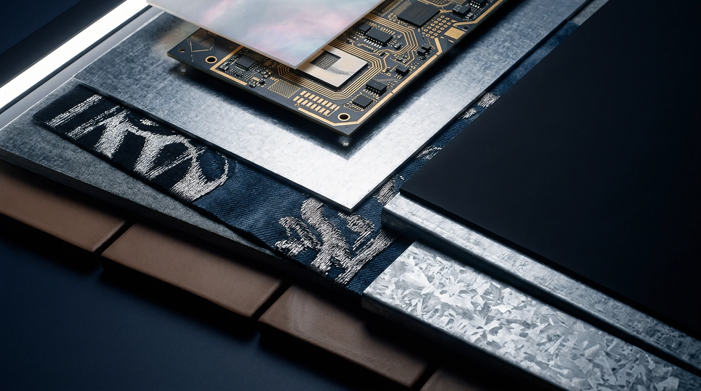
Ferromagnetic materials in the board stack distort surface magnetic fields. Electroless Nickel Immersion Gold finishes, for instance, deposit a ferromagnetic nickel layer containing three to eight percent phosphorus over surface copper features. The magnetic permeability of this nickel alters local flux lines, bending trace fields into asymmetric spatial profiles.
Additionally, continuous copper power planes generate eddy currents under AC excitation, screening magnetic field signals from deeper laminate layers.
Does Material Permeability Distort Inverted Current Density Profiles?
Static DC bias measurements eliminate eddy current screening in underlying copper planes while isolating purely resistive leakage from capacitive coupling currents. Alternatively, low-frequency AC lock-in scanning circumvents skin depth limits in inner copper planes, letting magnetic fields pass through laminate layers without amplitude loss. Mapping relative permeability across an unpopulated board provides a compensation matrix used to correct surface vector measurements before running linear matrix inversion routines.
Differential imaging strips away ambient trace fields when background noise threatens spatial resolution. Subtracting a golden reference board’s magnetic profile from that of a failing unit isolates the specific magnetic signature of the subterranean short circuit. Applying this differential technique across high-density interconnect designs pulls micro-ampere leakage signals directly out of multi-ampere power supply trace background fields.
- Connect the board under test to a stable programmable voltage source equipped with continuous precision current monitoring.
- Scan the unpowered reference board across the complete inspection region to map residual magnetic material signatures and environmental offset fields.
- Apply power bias below the thermal run-away threshold while modulating the excitation voltage with a 1 kilohertz reference carrier.
- Capture the active surface magnetic vector profile across the identical spatial grid points recorded during the reference scan.
- Subtract the baseline reference vector field from the active vector field to isolate net differential magnetic flux patterns.
- Filter spatial high-frequency noise using a spatial Gaussian low-pass kernel calibrated to the sensor standoff distance.
Inner-layer leakage escapes often reflect dielectric insulation failure inside glass-reinforcement weaves rather than non-repeatable board handling conditions.

Depth
Determining the vertical position z of an internal leakage current requires evaluating spatial frequency magnitude decay slopes across surface magnetic vector profiles. Magnetic field components emitted by horizontal current threads attenuate with spatial frequency k = sqrtkx2 + ky2 according to an exponential decay term e-k ztotal, where ztotal represents the sum of the physical sensor altitude z0 and the subterranean defect depth zfault. Taking the natural logarithm of the spatial field power spectrum yields a linear slope proportional to total depth, isolating the defect layer without physical microsectioning.
A 12-layer high-density interconnect PCB measuring 1.6 millimeters in total thickness contains a buried 45 microampere short circuit between power and ground vias. Scanning the surface magnetic field Bz(x,y) at a fixed sensor altitude z0 = 100 micrometers with a grid step size of 25 micrometers generates a 4000 × 4000 spatial matrix. Evaluating the logarithmic power spectral density along spatial frequency bands between 2 cycles per millimeter and 8 cycles per millimeter establishes a linear decay slope corresponding to a total source distance of 820 micrometers.
Subtracting the 100 micrometer sensor standoff distance positions the localized defect at depth z = 720 micrometers beneath the top surface laminate. This calculated depth matches layer 7 in the layer stack-up drawing, corresponding to the inner ground plane interface. Reconstructing the planar current vector field vecJ(x,y) at this specific plane depth reveals a sharp current convergence node where two adjacent inner traces converge near a buried via land.
Failure to meet the minimum ten microampere current sensitivity threshold defined in secondary diagnostic acceptance guidelines invalidates magnetic inversion proof for subterranean board returns.
Standard thermal imaging misses short circuits of this nature because thermal diffusion spreads heat laterally as energy conducts upward through FR-4 resin layers, expanding a 10 micrometer physical short into a diffuse 2 millimeter surface hotspot. Magnetic inversion preserves lateral coordinate precision regardless of depth, accurately pinpointing the spatial origin within 15 micrometers at layer 7 depth levels.
| Layer Depth (µm) | Lateral Accuracy (µm) | Depth Accuracy (µm) | Minimum Current (µA) | Scan Time (min) |
|---|---|---|---|---|
| 150 (Layer 2) | 3.5 | 8.0 | 5 | 12 |
| 400 (Layer 4) | 8.0 | 15.0 | 12 | 15 |
| 720 (Layer 7) | 15.0 | 28.0 | 45 | 22 |
| 1200 (Layer 10) | 32.0 | 55.0 | 110 | 35 |
| 1600 (Layer 12) | 50.0 | 85.0 | 250 | 45 |
Because field decay tracks altitude and spatial frequency windowing isolates high-frequency noise, the accuracy of vertical depth inversion hinges on precise standoff distance calibration. A 10 micrometer error in standoff height offsets layer depth assignments by an entire substrate dielectric layer.
According to standard electrical defect analysis guidelines under IPC-TM-650 Method 2.6.3.7, non-destructive isolation reports must establish defect spatial coordinates within a confidence radius smaller than the drill bit diameter used for physical sectioning before structural validation begins.
Proof
Inverted magnetic current density profiles require absolute structural verification before committing high-value PCB assemblies to destructive failure analysis procedures. Correlating non-destructive magnetic inversion coordinates with secondary analytical techniques prevents unneeded destruction of scarce prototype boards. Focused Ion Beam micro-milling and X-ray computed tomography rely on magnetic spatial coordinates to narrow down target volumes, cutting inspection times from days to hours.
High-resolution X-ray computed tomography validates internal metallic bridging when density differentials exist between copper filaments and surrounding resin glass substrates. When micro-ampere leakage paths consist of narrow, single-crystal copper dendrites under 500 nanometers in diameter, X-ray absorption contrast becomes insufficient for direct visualization. In these operational boundary conditions, magnetic field inversion remains the sole analytical method capable of isolating the defect coordinate frame.
Physical microsectioning without prior non-destructive magnetic spatial targeting routinely destroys subsurface conductive filaments before structural registration occurs.
Physical microsectioning cuts directly along the inverted current vector coordinates (x0, y0, z0) established during magnetic raster processing. Polishing the microsection plane in 1 micrometer steps while monitoring under scanning electron microscopy confirms the presence of conductive anodic filaments or subterranean copper slivers precisely at the predicted depth layer ~ confirming copper migration at layer six, while zero bias suppresses phantom peaks. Combining non-destructive spatial current density inversion with targeted metallurgical cross-sectioning delivers clear technical proof required to enforce supplier warranty claims or reject defective PCB manufacturing lots.
Validating non-destructive current localization maps against physical cross-sections transforms magnetic field inversion from an experimental diagnostic concept into a concrete delivery acceptance criterion across high-reliability electronics procurement contracts.