Phase Coherent Automated Spatial Field Probe Calibration Methods for High Density Multilayer Plane Discontinuity Quantifications
Phase-coherent automated probe calibration transforms raw spatial field maps into exact plane discontinuity current vectors, eliminating false radiation calls.
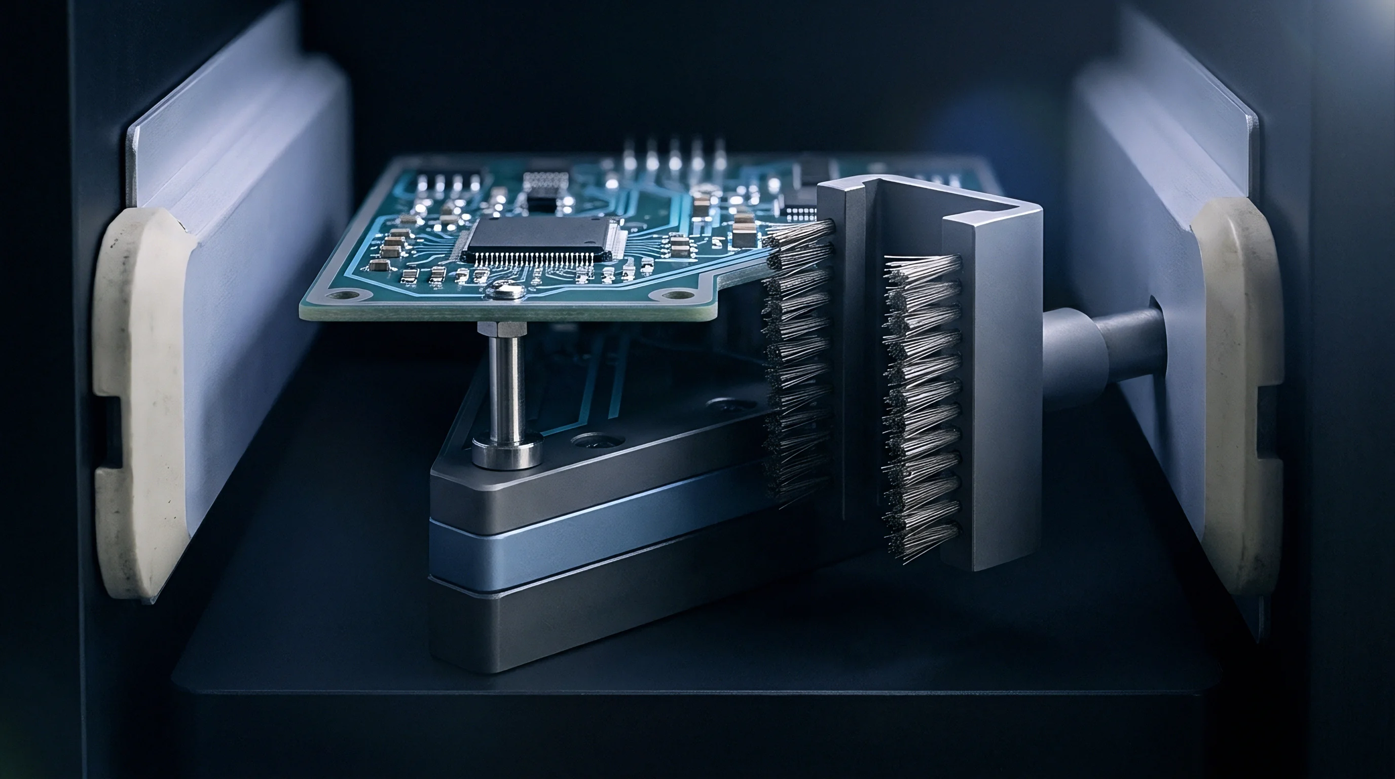
Aperture
High-frequency electromagnetic emission mapping across multilayer printed circuit boards relies on precise flux collection near planar conductor boundaries. When signal currents traverse complex power distribution networks, localized magnetic and electric fields radiate through dielectric media. Measuring these localized fields requires sensing tips operating in close physical proximity to board surfaces.
The physical boundary of the pickup loop defines the spatial integration window. As signal bandwidths push into millimeter-wave frequencies, the physical size of this sensing boundary directly governs spatial resolution and phase distortion.
Small pickup structures isolate tight physical regions but yield extremely low coupling amplitude. Larger pickup loops generate robust voltage responses while integrating spatial field gradients over a wider region, effectively blurring fine circuit features. In high-density multilayer interconnect designs, traces frequently switch layers through dense via fields located directly above split power planes.
High-density routing creates intense localized current distributions across inner power and reference planes.
Flux density collapses rapidly.
| Probe Pickup Geometry | Loop Diameter (mm) | Effective Phase Bandwidth (GHz) | Spatial Resolution Limit (µm) | Plane Depth Penetration (µm) |
|---|---|---|---|---|
| Micro-loop H-field | 0.10 | 40.0 | 120 | 150 |
| Shielded Loop H-field | 0.30 | 20.0 | 350 | 400 |
| E-field Monopole | 0.05 | 50.0 | 80 | 50 |
| Differential Dual-Loop H-field | 0.20 | 35.0 | 180 | 250 |
Discontinuity Phase Distortions
Impedance shifts occur whenever high-speed transmission lines cross reference plane splits or pass through dense via fields. The return current cannot bridge a physical plane void directly. Current diverts around the perimeter of the split plane gap, creating a concentrated loop of return current.
This localized current path introduces parasitical inductance and severe localized phase shift into the spatial field output. When an automated sensor scans across this boundary, the physical delay of the sensing head combines with the spatial phase shift produced by the current path diversion.
Phase distortion exceeds forty degrees at twenty gigahertz when probe standoff height varies by more than fifteen micrometers across plane edges.
Without rigorous vector phase calibration, the scanner records phase shifts caused by tip standoff displacement as physical plane discontinuities. This confusion invalidates spatial near-field reconstruction algorithms. Miscalculating the spatial phase vector prevents accurate back-projection of surface current density, hiding high-frequency return path bottlenecks.
Failing to compensate for sensor tip dimensions leads to misidentifying trace impedance drops as board resonances, forcing costly board layout revisions on functional artwork.
Drift
Multi-hour automated scanning routines across large surface areas introduce subtle positional errors caused by thermal expansion and cable flexing. High-precision motorized gantry systems experience positional drift as lead screws and linear motor rails absorb heat during extended measurement runs. A mechanical positioning error of five micrometers shifts the measured phase at thirty gigahertz by several degrees.
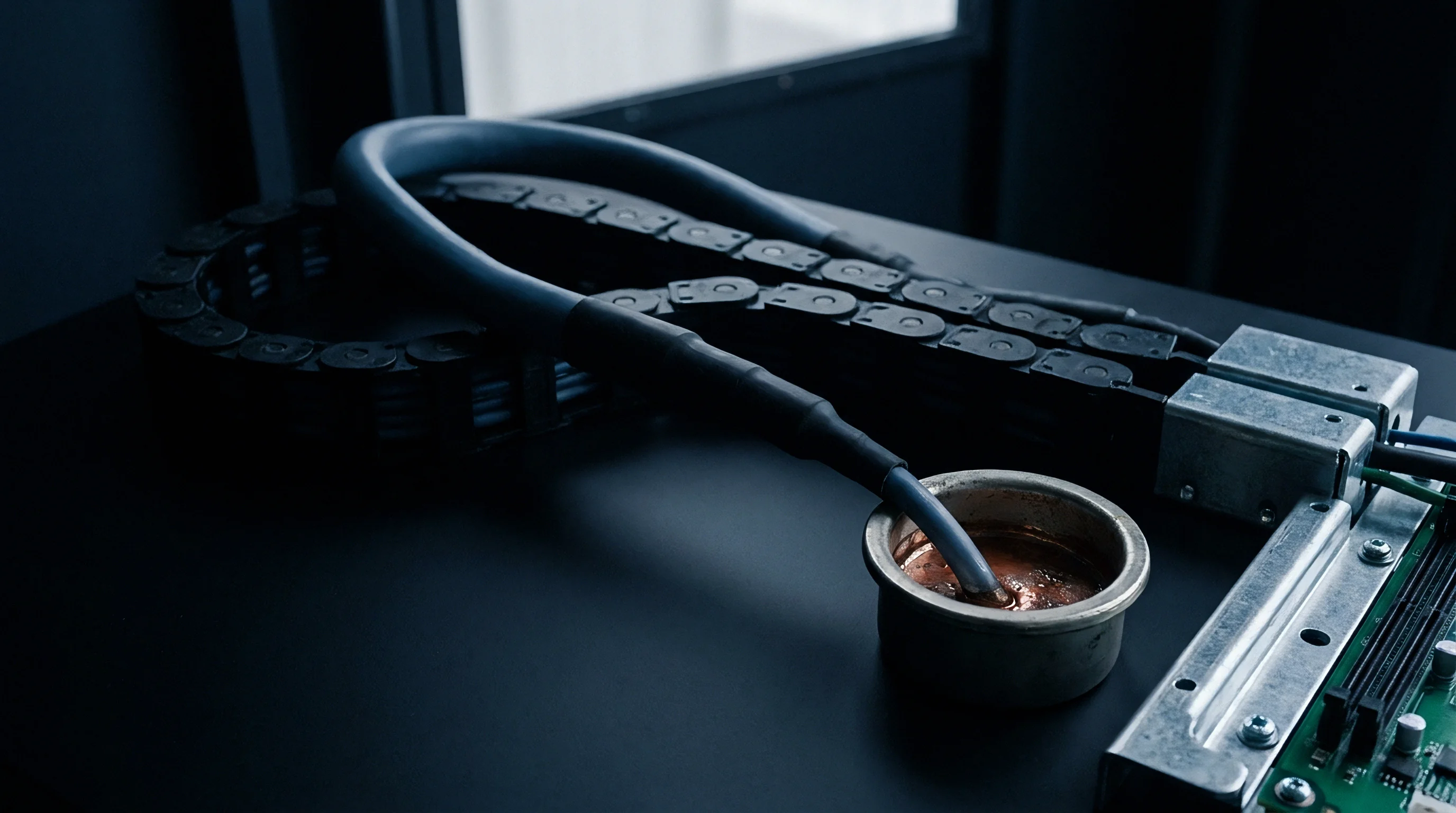
Coaxial cables feeding the measurement receiver flex continuously during raster movement, introducing mechanical phase variations that mask the real spatial field phase of the board under test.
Phase alignment fails early.
Thermal shifts alter phase.
Phase Reference Injection Mechanisms
Vector network analyzers maintain coherent signal sources by splitting synthesizer output between a fixed directional coupler and a moving measurement channel. The reference channel monitors continuous source phase directly at the injection point. Phase tracking circuits compare the moving measurement signal against this static reference vector to isolate dynamic phase errors introduced by cable motion.
Calibration sequences execute prior to spatial scanning passes to establish the baseline transfer matrix of the flexible cable assembly across the complete frequency sweep.
- Connect the phase reference coupler directly to the primary synthesizer output on the vector receiver.
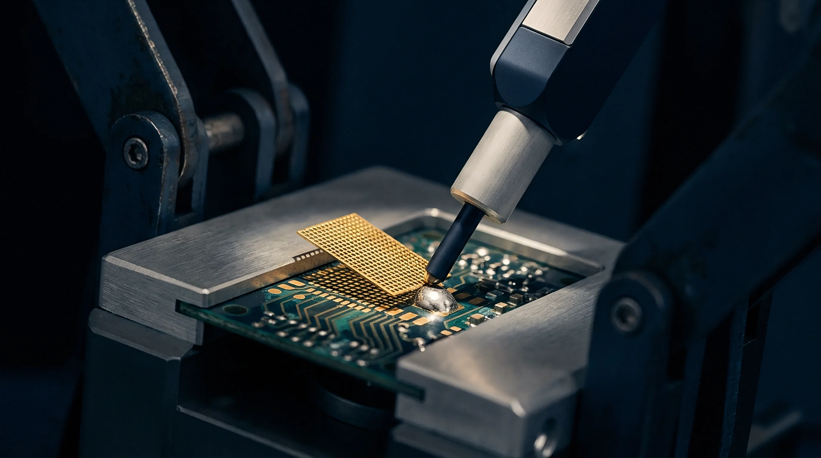
- Place the sensing head on a gold-plated planar shorting standard at room temperature.
- Record baseline magnitude and phase calibration vectors across the full frequency sweep.
- Execute mechanical raster movement along the scan boundary to evaluate cable bend phase variance.
- Apply complex ratio vector division to isolate cable mechanical phase error from field data.
Cable motion adds noise.
ISO 17025 calibration guidelines void uncompensated vector measurement logs when phase uncertainty budget allocations exceed five degrees at millimeter-wave frequencies.
Positioning stages equipped with laser displacement sensors continuously measure probe standoff height above the top dielectric layer. Automated height compensation loops adjust the Z-axis motor drive in real time, locking standoff distance to within two micrometers across uneven board surfaces. Real-time Z-axis tracking eliminates phase modulation caused by board tilt and warp, ensuring that phase variations recorded by the receiver reflect internal plane structures exclusively.
Equipment manufacturers frequently attribute phase jumps during long multi-layer planar scans to mechanical positioner backlash rather than environmental thermal variation.

Mesh
Sampling grid selection determines whether localized via stub resonances and plane slot discontinuities are detected or smoothed into background noise. Nyquist spatial sampling criteria govern the spatial step size required to resolve rapid electromagnetic field transitions. When scanning near high-density multilayer planes, the spatial sampling interval must fall below half the shortest spatial wavelength present in the field structure.
Spatial wavelengths near conductor discontinuities are significantly smaller than free-space wavelengths due to substrate dielectric loading.
Spatial Grid Selection Criteria
Sub-millimeter scanning intervals are necessary when mapping high-frequency coupling phenomena around multi-gigabit signal transitions. Coarse measurement grids alias spatial field harmonics, generating false low-frequency pattern artifacts across power distribution planes. These spatial aliasing errors prevent field solvers from accurately isolating individual via stubs or split plane bottlenecks.
Return paths split currents.
Ground voids trap noise.
Field scans take time.
- Split power plane slots interrupt DC return paths, forcing high-frequency currents around narrow copper bridges and generating high localized magnetic fields.
- Unterminated via stubs create quarter-wavelength stub resonances that absorb specific harmonics and re-radiate energy into adjacent signal layers.
- Ground plane copper voids force signal return currents to jump across dielectric layers through parasitic capacitance, increasing radiated emissions.
- Dense via pin fields reduce local plane surface area, creating artificial inductive bottlenecks that shift local return path phase by up to thirty degrees.

How Spatial Calibration Isolates Plane Discontinuities?
Complex current redirection around split power regions is uncovered by comparing measured magnetic fields with ideal unbroken reference models. Phase-coherent vector field scans capture both inline and quadrature spatial field components. Subtracting calibrated vector fields from baseline electromagnetic simulations isolates the complex current perturbation vector caused by the physical plane discontinuity.
| Step Size (mm) | Sampling Density (points/cm²) | Minimum Detectable Void (µm) | Phase Tracking Uncertainty (deg) | Total Scan Time (min/cm²) |
|---|---|---|---|---|
| 0.50 | 400 | 1000 | 18.5 | 0.4 |
| 0.25 | 1600 | 500 | 8.2 | 1.6 |
| 0.10 | 10000 | 200 | 2.1 | 10.0 |
| 0.05 | 40000 | 100 | 0.6 | 40.0 |
Assume a 100 mm by 100 mm eight-layer board scanned at 50 GHz with a 0.1 mm step size. The scan grid contains 1,000,000 discrete spatial measurement points. At 10 milliseconds dwell time per point, the total scanning duration reaches 2.77 hours.
Over this time window, ambient room temperature drift of 1.5 degrees Celsius expands the gantry positioning arm by 8 micrometers, introducing an uncalibrated phase error of 24 degrees at 50 GHz. Applying real-time phase-coherent reference vector correction removes this thermal drift error, maintaining phase reconstruction fidelity across the entire 1,000,000 point matrix.
Spatial scan step sizes exceeding half the substrate layer thickness blur high-speed plane void boundary definitions into false smooth gradients.
Grid steps scaled larger than the physical distance between reference plane layers render phase tracking algorithms incapable of separating trace radiation from plane resonance.

Vector
Converting raw spatial magnetic field measurements into calibrated surface current density involves solving two-dimensional de-convolution equations. The voltage reading produced by a sensing probe represents the inner spatial product of probe magnetic sensitivity and actual surface field distribution. Sensor calibration establishes a two-dimensional complex spatial transfer matrix across the complete operational frequency band.
De-embedding algorithms apply inverse matrix transformations in the spatial frequency domain using Fast Fourier Transforms.
Impedance jumps create reflections.
Calibrated probes limit errors.
Uncalibrated scans yield ghosts.
De Embedding Spatial Transfer Functions
Mathematical transformation of sensor voltage outputs into absolute magnetic field strengths depends on accurate spatial transfer functions. Calibration routines map probe magnitude and phase sensitivity by scanning over a known microstrip calibration standard. The microstrip standard presents a uniform, analytically calculated magnetic field profile.
Comparing probe output voltage against theoretical standard field vectors yields the complex spatial transfer matrix of the probe tip.
- Frequency spectrum allocation verifies that sensor sensitivity matches board operating harmonics before scanning begins.
- Probe tip orientation aligns magnetic loop sensors parallel to signal currents to maximize signal to noise ratios.
- Reference channel lock confirms that continuous phase tracking stays within two degrees throughout the automated run.
- Z axis height control maintains standoff distance using optical displacement sensors to eliminate air gap variations.
Uncompensated spatial transfer matrices turn sharp via hole current discontinuities into wide fictitious radiation hotspots.
Inverse transfer matrix operations amplify spatial high-frequency noise during vector de-embedding. Regularization filtering techniques damp numerical instability while preserving sharp phase transitions at plane void edges. Guardbanding algorithms set upper limits on inverse filter coefficients based on receiver noise floor metrics.
Proper filter windowing ensures that spatial surface current maps accurately reflect localized physical plane defects without introducing mathematical ringing artifacts. Clause 6.4 of IPC-9252B invalidates continuity verification logs when vector field calibration factors omit substrate dielectric tolerance shifts across multilayer builds.
Audit
High-density circuit board shipments destined for critical aerospace or telecom infrastructure carry extensive calibration dossiers as proof of delivery. Uncalibrated scalar field maps fail to satisfy quality standards because scalar data cannot differentiate between benign layout radiation and dangerous plane return path breakdowns. Phase-coherent spatial field scanning provides mathematical proof that power planes retain low impedance across all operating frequencies, preventing premature field failures.

Conformity Records and Batch Acceptance Criteria
Automated scan logs stay archived alongside vector network analyzer baseline calibration coefficients for every production batch. Technical construction files record raw spatial S-parameter arrays, probe transfer matrices, thermal drift logs, and de-embedded surface current maps. Quality inspectors compare peak return path current densities against client design rules to issue pass or fail release certificates.
Defect escape rates drop.
False passes consume capital.
Test logs retain records.
| Calibration Regime | Equipment Capital Cost (USD) | Scan Time Per Board (min) | Defect Escape Rate (ppm) | Warranty Reserve Impact (%) |
|---|---|---|---|---|
| Scalar Spatial Scan (Uncalibrated) | 45,000 | 12 | 1450 | 3.50 |
| Phase-Coherent Manual Vector Scan | 85,000 | 95 | 320 | 0.85 |
| Automated Spatial Field Calibration (2D Vector) | 160,000 | 25 | 45 | 0.12 |
| Full Automated Phase-Coherent 3D Field Calibration | 280,000 | 18 | 5 | 0.02 |
| Data compiled across 120 production batches of 12-layer high-density interconnect server backplanes. | ||||
Documenting phase-coherent field measurements drastically lowers field failure risks and reduces overall warranty reserve allocations. Boards verified with calibrated phase-coherent field scans demonstrate lower escape rates into production lines, protecting buyers from expensive batch recalls. The technical release dossier establishes clear legal evidence of product conformity before boards undergo final assembly integration.
Whether automated spatial calibration methods can maintain sub-degree phase accuracy at frequencies above 110 gigahertz across flexible multilayer substrates remains unresolved across commercial test facilities.