Modeling High Frequency Signal Attenuation Caused by Parasitic Test Point Capacitance across Multilayer PCB Traces
Test point parasitic capacitance creates localized low-impedance discontinuities that increase insertion loss and jitter on high-speed PCB traces.


Stub

Discontinuity Mechanics at High Data Rates
Adding an exposed copper test pad to a high-speed transmission line loads that region with extra capacitance to ground, dropping the trace’s characteristic impedance across the landing area. Once the signal wavelength shrinks to about twenty times the combined length of the pad and its via transit, the discontinuity stops behaving as a pure lumped element and transitions into a distributed wave interaction. On serial links running above ten gigabits per second, even a hundred-femtofarad parasitic tap distorts phase linearity, adds deterministic jitter, and carves steep notches into the insertion loss curve.
Test point capacitance comes from three main sources: the surface pad facing the reference plane, the vertical via barrel traversing layers, and any unused via stub left by incomplete drilling. Outer-layer microstrips put the pad right above the ground plane, maximizing parallel-plate capacitance. Striplines route the signal through an inner layer, so reaching a test point requires a blind or thru-hole via that acts like an open-ended stub.
At the frequency where this stub reaches a quarter-wavelength electrically, its input impedance drops to zero, pulling signal energy directly off the main trace.
An un-etched test point stub acting as a quarter-wave resonant structure creates an operational stop-band notch that completely suppresses signal transmission at its resonant frequency.
At the test point itself, performance turns on how far local impedance drops below nominal. Loading a fifty-ohm trace with an abrupt two-hundred-femtofarad capacitance can pull impedance down to thirty-five ohms or less across the pad span. The step changes at the entry and exit of this region trigger partial reflections.
Energy bounces back and forth within the discontinuity before leaking back into the main signal path delayed, degrading signal amplitude at the receiver while compounding inter-symbol interference.
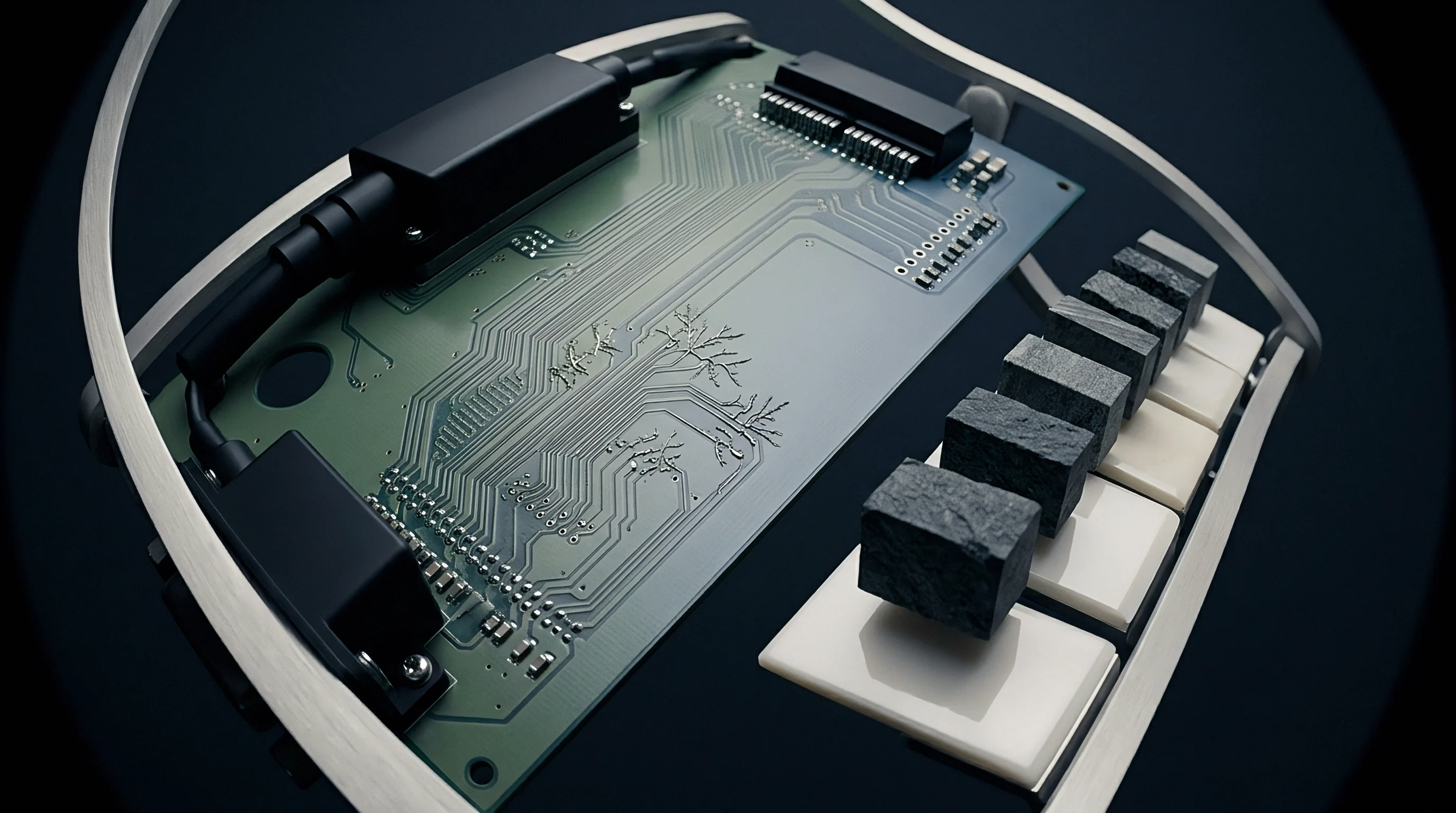
Reflectometry Dynamics and Impedance Dips
Time-domain reflectometry spots both the location and reactive behavior of the test pad. Sending a step impulse with a five-picosecond rise time down the trace produces a negative voltage trough at the test point. The depth of that dip scales with total lumped capacitance, while its width reflects the physical delay through the pad combined with the rise time of the measurement edge.
On high-permittivity substrates, sub-millimeter layout details change the shape of this voltage trough dramatically. Slower signals with two-hundred-picosecond edges average out the discontinuity across their wavefront, producing small reflections that hardly alter the eye diagram. Channels with edge rates under twenty picoseconds resolve fractions of a millimeter across the landing area; their high-frequency spectral content sees the full parallel capacitance, scattering energy backward instead of letting it pass.
Calculating attenuation means modeling the test point as an asymmetrical pi- or T-network within the transmission line. The shunt leg combines parallel-plate capacitance, perimeter fringe fields, and via barrel capacitance. High-frequency signals see an impedance formed by the trace impedance in parallel with the pad’s capacitive reactance.
As frequency climbs, that reactance falls, shunting more signal current to ground before it ever reaches the receiver.
Limiting this current loss while retaining probe access takes careful layout around the pad and reference layers. Cutting out ground plane copper under the pad increases the spacing to the return plane, cutting broadside capacitance but adding loop inductance. If return currents have to detour around wide plane voids, the discontinuity turns into a tank circuit that rings at high frequencies and degrades the signal-to-noise ratio.
High-speed differential design rules tightly cap stub length and pad parasitics to protect operating margins. Adding an un-tuned test pad to a twenty-eight gigabit per second NRZ or fifty-six gigabit per second PAM4 trace closes the eye beyond usable limits. Every probe point added for bed-of-nails or flying-probe access acts as a reactive load, consuming dynamic margin out of the total channel loss budget.
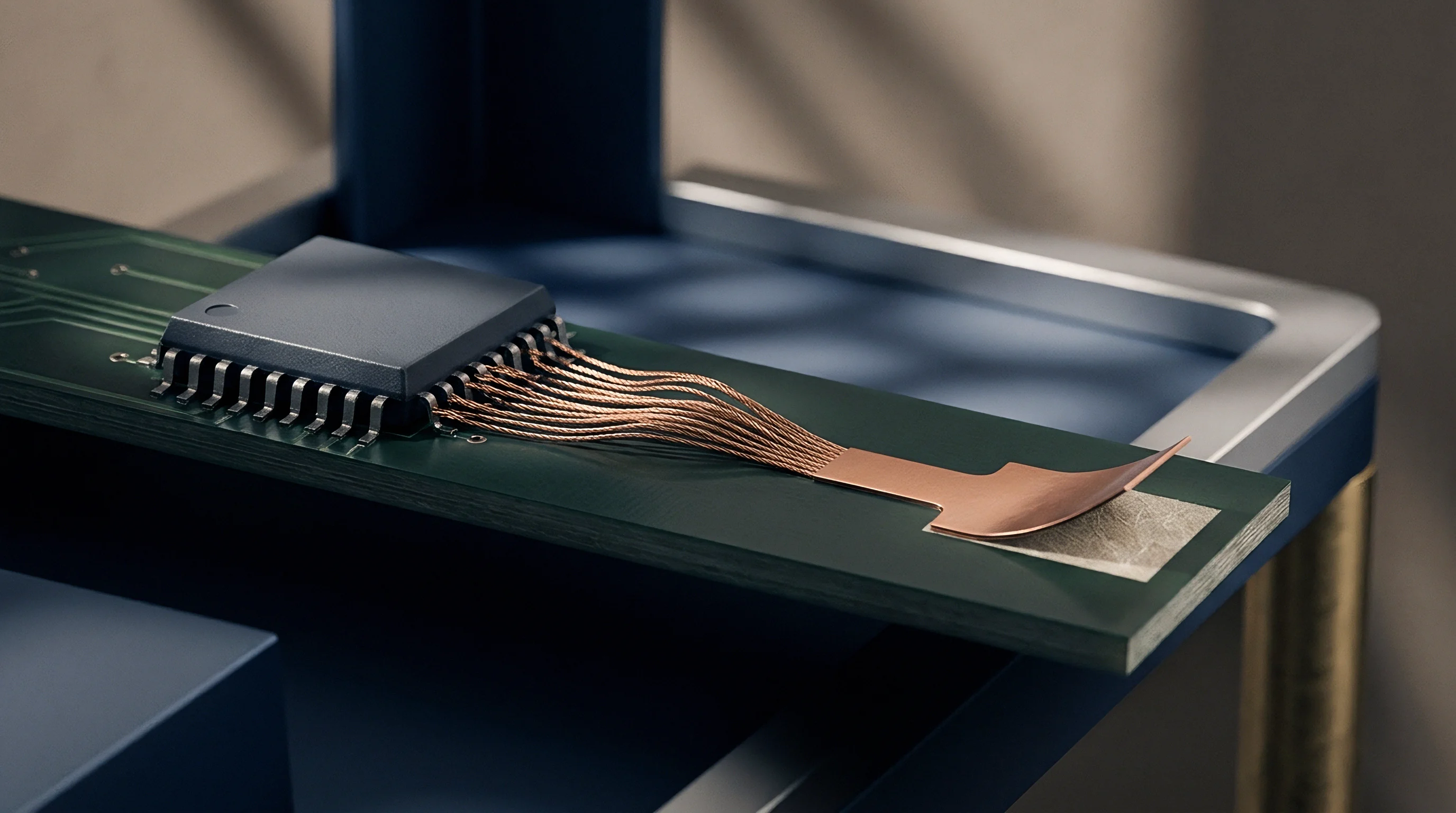
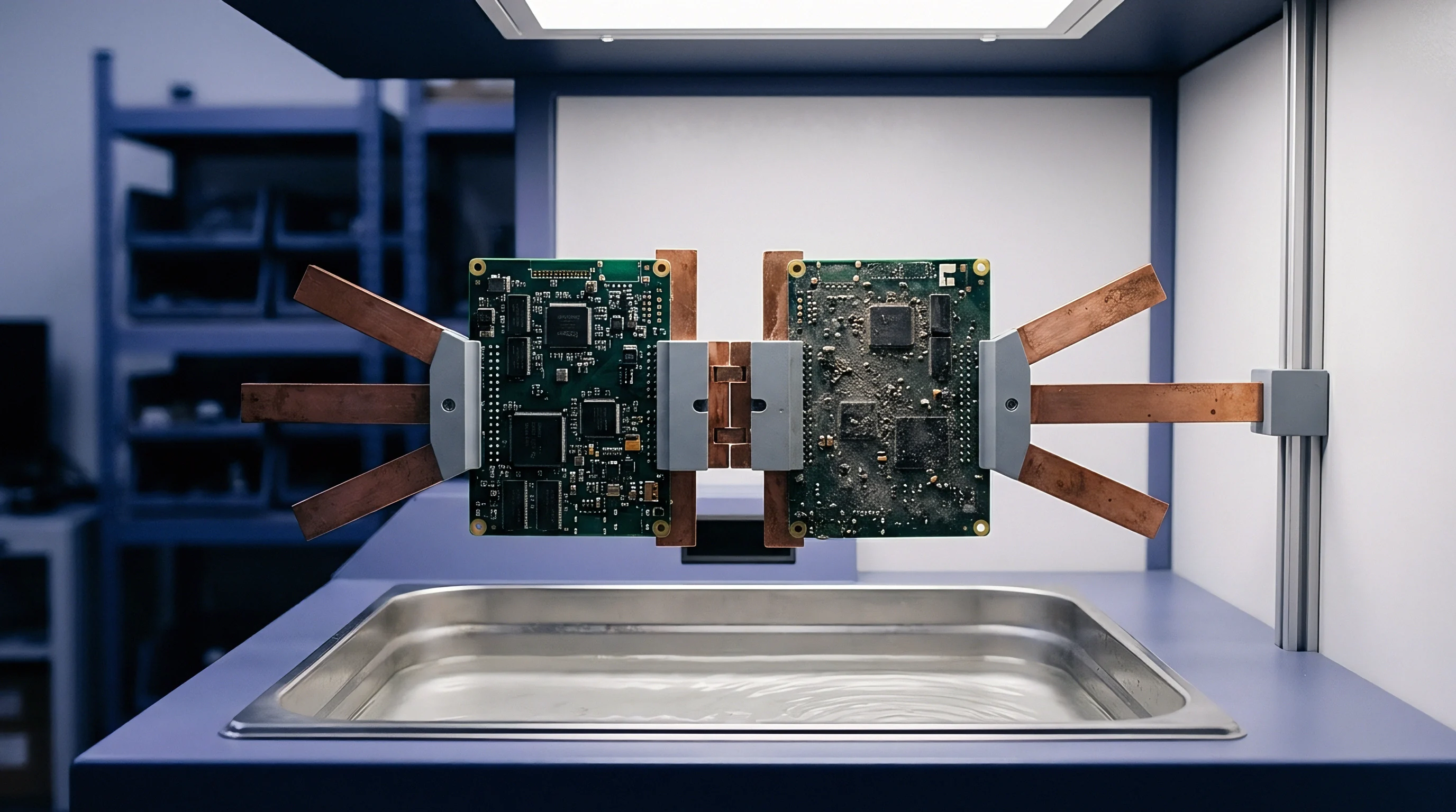
Matrix

Transmission Parameters and Network Cascading
Evaluating high-frequency loss along a trace with parasitic test points requires converting physical geometries into two-port scattering parameters. A uniform trace of length L is defined by its characteristic impedance and propagation constant, producing a basic transfer matrix. Adding parasitic capacitance splits that trace into two line segments on either side of a lumped shunt admittance.
Converting each section’s S-parameters into ABCD cascade matrices allows matrix multiplication to yield the full channel response.
The shunt admittance of the test point contains both conductive and reactive terms. Assuming negligible dielectric loss across the small volume of the pad, admittance reduces to the dynamic frequency term multiplied by total parasitic capacitance. Applying Kirchhoff’s circuit laws gives the ABCD matrix for a purely lumped shunt admittance on a line:
A equals 1, B equals 0, C equals j multiplied by 2, multiplied by pi, multiplied by frequency, multiplied by parasitic capacitance, and D equals 1.
Multiplying the input trace segment matrix by the shunt admittance matrix, then multiplying by the output segment matrix, gives the overall system response. Converting this composite ABCD matrix back to two-port S-parameters yields analytical expressions for insertion loss (S21) and return loss (S11). The cascaded calculation shows that attenuation scales non-linearly with frequency and depends strongly on how close the test point sits to terminations or other impedance steps.
Network cascading pinpoints where parasitic capacitance begins dominating channel performance. The S21 expression reveals a first-order pole created by the shunt capacitor reacting against the parallel combination of source and load impedance. In a matched fifty-ohm system, source and load present an effective twenty-five-ohm parallel resistance across the pad.
The three-decibel corner frequency falls where capacitive reactance matches this twenty-five-ohm value.
Worked Attenuation Derivation for Scaled Parasitics
A practical example shows how minor layout features cause electrical failure. Take a differential channel running at a fourteen-gigahertz clock frequency to support twenty-eight gigabit per second NRZ data. The single-ended trace impedance is fifty ohms.
A surface test point adds three hundred femtofarads of parasitic capacitance from pad area, fringe fields, and an un-drilled blind via stub. Computing the insertion loss penalty at fourteen gigahertz relies on the lumped-shunt equation derived from the cascaded ABCD matrix.
Calculating capacitive reactance at fourteen gigahertz yields one divided by two times pi times fourteen times ten to the ninth hertz times three hundred times ten to the minus fifteen farads. That evaluates to roughly thirty-seven point nine ohms of capacitive reactance. The insertion loss magnitude for a shunt capacitor in a matched source and load system with characteristic impedance Z0 equal to fifty ohms follows the standard transmission ratio formula:
S21 magnitude equals one divided by the square root of the sum of one plus the square of the quantity Z0 divided by two times Xc.
Substituting fifty ohms for Z0 and thirty-seven point nine ohms for Xc gives an inner ratio of fifty divided by two times thirty-seven point nine, or fifty divided by seventy-five point eight, which equals zero point six six. Squaring that gives zero point four three five. Adding one leaves one point four three five under the radical, whose square root is one point one nine eight.
Dividing one by one point one nine eight gives an S21 amplitude magnitude of roughly zero point eight three five.
Converting this amplitude ratio into decibels via twenty times the logarithm base ten of zero point eight three five yields an insertion loss penalty of minus one point five six decibels at fourteen gigahertz. At the third harmonic of forty-two gigahertz ~ essential for fast edge transitions ~ capacitive reactance drops to twelve point six ohms. Recalculating loss at forty-two gigahertz gives an amplitude ratio of zero point four three six, representing an attenuation penalty of minus folded seven point two1 decibels from the test point alone.
| Parasitic Capacitance (fF) | Frequency (GHz) | Capacitive Reactance (Ohms) | Calculated S21 Loss (dB) | Equivalent TDR Impedance Dip (Ohms) |
|---|---|---|---|---|
| 100 | 5.0 | 318.3 | -0.05 | 46.2 |
| 100 | 14.0 | 113.7 | -0.38 | 46.2 |
| 100 | 28.0 | 56.8 | -1.37 | 46.2 |
| 250 | 5.0 | 127.3 | -0.31 | 41.5 |
| 250 | 14.0 | 45.5 | -2.14 | 41.5 |
| 250 | 28.0 | 22.7 | -5.46 | 41.5 |
| 500 | 5.0 | 63.7 | -1.16 | 35.1 |
| 500 | 14.0 | 22.7 | -5.46 | 35.1 |
| 500 | 28.0 | 11.4 | -11.23 | 35.1 |
This attenuation occurs at a single point on the trace. If layout requirements place several test points along the same line for in-circuit bed-of-nails probing and boundary-scan nodes, loss compounds quickly. Regularly spaced capacitive loads turn the line into a periodic slow-wave structure, acting like a low-pass Bragg filter with sharp stop-bands that block high-frequency content and collapse the eye.
Amplitude attenuation comes with phase distortion. The imaginary term of the composite ABCD matrix introduces group delay ripple across the spectrum, causing different spectral components of the data pulse to travel at different phase velocities through the pad area. This dispersion spreads energy into adjacent unit intervals, producing inter-symbol interference that receiver continuous-time linear equalization (CTLE) cannot clean up.
Accurate analysis past initial estimations uses three-dimensional electromagnetic field solvers rather than simple lumped models. Solvers solve boundary conditions across the volume around the pad, capturing fringe capacitance through dielectric layers and to neighboring traces. Importing these extracted S-parameters into transient bit-by-bit or statistical simulators maps eye degradation, jitter buildup, and bit-error-rate floors under operational conditions.
High-speed compliance standards enforce strict limits on channel insertion loss across the Nyquist band. Standards like IEEE 802.3 for Ethernet or PCIe Base Specifications prohibit layout access points from pushing total channel transmission outside the defined loss mask.
Compliance verification also touches contractual artwork approvals. Per IPC-2221 section 5.2.3, adding an un-modeled conductor to a controlled-impedance trace voids the impedance tolerance guarantees signed off on the fabrication artwork.

Stackup

Layer Topologies and Field Distribution
Where a high-speed trace sits in a multilayer board stackup dictates its sensitivity to test point parasitics. Outer microstrip traces have air above and substrate below, creating an asymmetrical field with an effective dielectric constant below the bulk material value. Adding a surface test pad requires widening the copper trace to fit a mechanical probe tip.
That extra broadside surface area generates substantial parasitic capacitance to the reference plane directly underneath.
Inner striplines sit completely in dielectric, sandwiched between two ground planes. Probing a stripline requires bringing the signal up to the surface with a vertical via, breaking the uniform field structure of the buried trace. The via barrel adds series inductance, while the surface pad and inner capture rings add parallel capacitance to every reference plane the via pierces.
Total parasitic loading on a stripline test point comes from both the surface landing pad and the vertical via assembly.
According to IPC-2141 guidelines for high-speed controlled impedance board design, removing reference plane copper directly beneath a surface feature lowers local parasitic capacitance while increasing loop inductance and EMI radiation risks.
Managing capacitance in high-density stackups often involves etching out ground copper directly beneath the surface test pad. Removing reference metal on the layer right under the point creates a localized void, increasing the distance to the nearest return path. Broadside capacitance drops proportionally as spacing increases, forcing electric field lines to fringe over longer paths toward deeper ground layers or surrounding coplanar copper.
Removing ground copper under test points alters localized impedance in ways that require tight control during manufacturing. Common layout strategies for tuning this impedance profile include:
- Reference Plane Relief Voiding expands the ground plane opening beneath the pad, reducing parallel plate capacitance while raising local characteristic impedance toward target values.
- Antipad Diameter Optimization enlarges the clearance ring surrounding via barrels on inner reference planes, suppressing capacitance between the barrel and inner ground layers.
- Deep Blind Via Drilling removes the open-ended copper stub remnant extending past the inner-layer stripline destination, suppressing quarter-wave resonant notches inside the operational band.
- Coplanar Ground Shielding pulls coplanar ground traces back from the test pad perimeter, controlling edge-to-edge fringe capacitance on outer routing layers.
Opening up plane relief involves trade-offs between return path continuity and EMI performance. When reference copper is carved out under a test point, return currents must loop around the void’s edge, raising local loop inductance. While balancing capacitance against inductance can bring localized trace impedance back to fifty ohms, the enlarged current loop generates common-mode noise, increasing radiated emissions and leaving the trace vulnerable to crosstalk.

Dielectric Variations and Stackup Interactions
Substrate selection sets the overall scale of parasitic capacitance across temperature and frequency. Standard FR-4 epoxy laminates have a dielectric constant near four point two at one gigahertz, drifting down at higher frequencies. High-speed laminates using specialized resins and low-profile foils run between two point seven and three point five.
Moving to a lower-permittivity substrate reduces parasitic capacitance for a given pad geometry in direct proportion to the drop in dielectric constant.
| Stackup Routing Type | Substrate Dielectric Constant (Dk) | Test Pad Surface Area (sq mm) | Ground Relief Void Included | Total Parasitic Capacitance (fF) | Bandwidth Limit (-1dB S21 GHz) |
|---|---|---|---|---|---|
| Outer Microstrip | 4.3 (Standard FR-4) | 0.50 | No | 380 | 9.2 |
| Outer Microstrip | 4.3 (Standard FR-4) | 0.50 | Yes (Layer 2 Void) | 190 | 18.4 |
| Outer Microstrip | 3.0 (Low-Loss PTFE) | 0.50 | No | 265 | 13.2 |
| Outer Microstrip | 3.0 (Low-Loss PTFE) | 0.50 | Yes (Layer 2 Void) | 130 | 26.8 |
| Embedded Stripline + Via | 3.7 (Mid-Loss Epoxy) | 0.35 | No | 420 | 8.3 |
| Embedded Stripline + Via | 3.7 (Mid-Loss Epoxy) | 0.35 | Yes (Layers 2/3 Void) | 210 | 16.6 |
Dielectric thickness determines what trace width achieves target impedance. Thin outer cores bring the reference plane close to the microstrip, requiring narrow trace widths for a fifty-ohm match. Adding a fixed-size test pad over a thin core creates a large capacitive spike because the dielectric gap in the parallel-plate equation is small.
Thicker outer dielectrics shrink that spike, but demand wider trace routing across the entire board, cutting into available routing density.
Managing high-speed test access requires balancing physical probe needs against high-frequency limits. Fabrication houses often flag aggressive relief patterns during pre-production audits, as large ground voids beneath test points can compromise mechanical layer stability and cause localized impedance variations during lamination.
Holding signal loss within budget while preserving structural integrity requires tight fabrication tolerances. Variations in prepreg thickness, resin content, and copper plating change real-world parasitic numbers. A ten percent drop in dielectric thickness paired with a ten percent increase in copper plating raises pad capacitance by over fifteen percent, pushing a marginal channel into failure.
Bench

High-Frequency Measurement Protocols
Validating analytical loss models takes bench measurements with calibrated instrumentation. A Vector Network Analyzer (VNA) measuring two-port or four-port differential S-parameters extracts insertion loss, return loss, and phase behavior over frequency. Because connecting coaxial cables to thin PCB traces adds fixture losses and reflections, de-embedding algorithms must strip out launch and connector effects to reveal true trace performance.
Time-Domain Reflectometry (TDR) complements frequency sweeps by mapping impedance directly along the length of the trace. TDR instruments launch step pulses with picosecond rise times down the line, recording reflected voltage against propagation time. A parasitic test point shows up as a sharp dip in the impedance profile.
Integrating the area of that dip yields the lumped capacitance added by the pad, giving clear empirical data to calibrate layout extraction tools.
Accurate de-embedding relies on dedicated calibration structures built onto the test coupon. Common de-embedding methods for high-frequency board testing include:
- Thru-Reflect-Line (TRL) Calibration utilizes precise transmission line standards fabricated on-board to shift the measurement reference plane directly to the input and output edges of the test point layout.
- Automatic Fixture Removal (AFR) extracts two-port S-parameters of the launch fixtures using time-domain gating, mathematically removing connector launches and access traces from measured data.
- Short-Open-Load-Thru (SOLT) Calibration establishes baseline instrument calibration at the coaxial cable tips, requiring subsequent mathematical subtraction of port launch parasitics via S-parameter matrix de-embedding.
Small probing errors distort extracted parasitic values. Inconsistent needle pressure alters contact resistance and adds parasitic loop inductance. Poor grounding on coplanar microprobes creates ground loops that appear on VNA sweeps as artificial resonance notches, making test point attenuation look worse than it is.
What Dynamic Range Remains after Fixture Deembedding?
Dynamic range after fixture de-embedding depends on the network analyzer’s noise floor and launch fixture loss. If a test fixture drops signal by twenty decibels at forty gigahertz, mathematically removing that fixture boosts trace noise by twenty decibels. That loss of dynamic range makes it difficult to resolve tiny insertion loss steps ~ like a zero-point-three-decibel drop from a small pad ~ above background noise.
Isolating a single test point along a long trace requires time-domain gating, which applies a mathematical window to filter out reflections from connectors and terminations. Setting that window too narrow clips the capacitor’s impulse response, smoothing out the impedance dip and understating attenuation. Setting it too wide captures secondary reflections from board edges, skewing the S21 phase measurement.
Matching bench data to 3D field solver models uncovers physical effects that 2D tools miss. For instance, an unexpected resonance observed during testing often comes down to an un-drilled via stub left when controlled-depth back-drilling misses its specified five-mil length limit.
Skipping physical coupon validation creates serious commercial risk in volume production. Boards that pass low-frequency bed-of-nails checks can systematically fail in high-speed operation, triggering costly recalls, scrapped inventory, and redesign delays.


Margin
Coverage Allocation and Design Rules
Test coverage requirements conflict directly with high-speed signal integrity budgets. Manufacturing teams want maximum nodal access for In-Circuit Testing (ICT), flying probe inspection, and boundary scan to catch solder bridges, opens, and incorrect components early. Signal integrity engineers, meanwhile, want zero stubs and minimal capacitive loading on high-speed traces to preserve eye openings and timing margins.
Balancing these priorities takes a strict access budget matched to channel data rates. Low-speed control lines, power nets, and reset signals easily tolerate test points with several picofarads of parasitics without issue. Serial links running above ten gigabits per second must severely limit test pads, relying instead on non-intrusive testing like IEEE 1149.6 boundary scan and built-in loopback diagnostics.
Where physical probe access is unavoidable on medium- to high-speed traces, explicit layout rules limit performance impact. Standard practices for high-density interconnects include:
- Micro-Pad Dimensioning restricts test pad landing diameters to small probe target limits, reducing physical surface area and broadside parallel plate capacitance.
- Differential Symmetry Preservation forces test point additions on differential pairs to be placed as mirror-image structures on both legs, preventing differential-to-common mode conversion.
- Orthogonal Stub Alignment aligns via transitions and pad extensions perpendicular to the primary transmission vector, minimizing magnetic coupling into adjacent traces.
- Keep-Out Zone Enforcement removes coplanar copper fills and adjacent trace routing within three pad radii of the test target to eliminate uncontrolled fringe coupling.
Deciding whether to remove test points requires quantifying lost fault coverage. Stripping probe pads from a sixteen-lane PCI Express bus removes thirty-two nodes from the in-circuit test fixture. That drops traditional bed-of-nails fault coverage on those nets to zero percent, pushing defect screening entirely onto optical inspection and high-speed boundary scan.
Boundary-scan testing under IEEE 1149.6 uses AC-coupled signals to verify differential high-speed continuity without probe pads. Boundary cells built into transceiver silicon drive pulses through coupling capacitors, detecting opens and shorts via internal registers. Using AC boundary scan restores structural test coverage while leaving traces unencumbered by test pads.

Yield Trade-Offs and Financial Exposure
The tension between physical test access and signal loss shows up directly on the bottom line. Eliminating all test points to protect signal margins moves defect detection downstream into functional or system-level testing. Catching an open joint during functional testing costs far more per unit than catching it at an unpowered ICT station, driven by diagnostic labor, longer test times, and risk of damaging downstream components.
On the flip side, scattering test points across high-speed lines creates a systematic yield problem. Boards that clear unpowered ICT can consistently fail functional eye-diagram checks from the added insertion loss and jitter. Scrapping or reworking fully populated boards because test pads degraded channel margins destroys manufacturing yield, wiping out whatever was saved on in-circuit testing.
Building guard bands into high-frequency layout rules prevents these yield losses. Designers model worst-case parasitic capacitance across dielectric tolerance bounds and include that attenuation directly in the loss budget. If operating margin with test points falls below protocol requirements, the pads are removed or converted to micro-vias for flying-probe access.
Friction between test development and signal integrity often stalls layout release. Test engineering pushes for full nodal access to meet factory quality metrics, while signal integrity specialists withhold sign-off on layouts carrying capacitive discontinuities on critical traces.
What structural metric determines the threshold where non-intrusive boundary-scan coverage fully offsets the field failure risks of removing physical bed-of-nails test points from high-speed differential traces?