Temperature Dependent Anisotropy Ratio Variations in Glass Reinforced Hydrocarbon Laminates at Millimeter Wave Frequencies
Thermal expansion alters resin density, driving dynamic anisotropy shifts that detune millimeter-wave phase stability and coupling tolerances across temperature.
Core
In high-frequency circuit boards, electromagnetic field behavior depends heavily on the arrangement of reinforcing fibers and resin matrix. Hydrocarbon laminates reinforced with woven E-glass or NE-glass exhibit pronounced dielectric anisotropy across millimeter-wave frequencies from 24 GHz to 110 GHz. This directional divergence stems directly from the composite geometry: high-permittivity glass yarns lie horizontally within a lower-permittivity hydrocarbon polymer loaded with ceramic filler particles.
Consequently, relative permittivity measured perpendicular to the board surface differs from that measured parallel to the plane, establishing an anisotropy ratio defined as the z-axis relative permittivity divided by the in-plane relative permittivity.
Thermal expansion in hydrocarbon resins alters matrix density, shifting dielectric properties along each spatial axis. At millimeter-wave frequencies, where physical trace widths shrink to sub-millimeter scales, even subtle changes in directional permittivity alter phase velocity, characteristic impedance, and coupling ratios. While older design workflows treated laminates as isotropic using single dielectric constants from datasheets, modern 77 GHz automotive radar and 60 GHz or 80 GHz wireless backhaul systems detune when temperature swings shift individual tensor permittivity components independently.

Tensor Permittivity and Spatial Heterogeneity
Because woven reinforcement fibers lie in the horizontal plane, in-plane dielectric properties diverge from out-of-plane values. Modeled as a tensor, relative permittivity breaks into three orthogonal components aligned with the weave’s longitudinal, transverse, and vertical axes:
barbarvarεr = beginbmatrix varεr,x & 0 & 0 \ 0 & varεr,y & 0 \ 0 & 0 & varεr,z endbmatrix
In standard woven laminates, warp and fill threads line up with the x- and y-axes in the board plane. E-glass carries a relative permittivity around 6.1, whereas cured hydrocarbon resin sits near 2.3 to 2.5, so electric fields aligned with the yarn bundles encounter higher bulk capacitance than fields running perpendicular to them. Adding amorphous silica or titanium dioxide fillers brings matrix permittivity up toward target values between 3.0 and 3.5, though filler particles tend to settle in resin pockets between bundles, preserving microscopic field asymmetry.
These tensor coefficients govern field propagation across different circuit topologies. Microstrip lines project electric fields vertically from trace to ground plane, aligning the primary vector with the z-axis while fringing fields extend into the x-y plane. Coplanar waveguides and edge-coupled differential pairs, by contrast, store a significant portion of their electric energy horizontally along the x- or y-axis.
Consequently, microstrips depend heavily on z-axis permittivity, whereas coplanar and edge-coupled structures respond to a combination of in-plane and out-of-plane values. This anisotropy ratio drives even- and odd-mode velocity mismatch in differential pairs, directly influencing eye closure and mode conversion at 56 Gbps and higher speeds.
The spatial orientation of woven glass yarns creates an inherent directional split between out-of-plane and in-plane permittivity that increases with reinforcement fabric weight.

Woven Glass Geometry and Resin Matrix Dynamics
Commercial laminates commonly use glass fabric styles such as 106, 1080, or 2116 impregnated with thermoset cross-linked polymers and ceramic filler. Fabric geometry defines the structural boundaries for anisotropy: lighter styles like 106 feature fine, tightly twisted yarns with open spacing, yielding lower bulk anisotropy but greater local variations in resin content, while heavier styles like 2116 rely on thicker yarn bundles that create distinct dielectric contrasts between glass-rich knuckles and resin-filled windows.
Mixture models capture how fields sample these composite structures. In-plane dielectric constant follows a parallel capacitive model, while z-axis permittivity behaves more like a series capacitive arrangement:
varεr,xy = vg varεg + vm varεm
frac1varεr,z = fracvgvarεg + fracvmvarεm
Here, vg represents glass fabric volume fraction, vm is the combined matrix and filler volume fraction, varεg is the glass dielectric constant, and varεm is the matrix dielectric constant. Because the series model places the low-permittivity matrix phase in series with high-permittivity glass, measured z-axis relative permittivity is consistently lower than in-plane permittivity. On a typical hydrocarbon core with 45 percent glass volume, z-axis relative permittivity might measure 3.48 at 10 GHz while in-plane permittivity along the warp yarn reaches 3.65, producing an initial anisotropy ratio of 0.953.
Uncorrected shifts in this spatial dielectric structure degrade microwave performance across high-density interconnect layers in several distinct ways:
- Phase velocity dispersion degrades antenna array beam-steering accuracy across broad frequency sweeps.
- Differential pair skew occurs when traces sit over changing proportions of glass bundles and resin pockets.
- Characteristic impedance drift shifts transmission line impedance off target, triggering reflections.
- Resonant frequency detuning pulls down bandpass filter center frequencies and narrowband matching networks.
- Mode conversion expansion increases crosstalk and electromagnetic radiation from high-speed differential channels.
The degree of spatial variation depends on laminate fabric style, ceramic filler loading, and press conditions during lamination. As operating frequencies reach millimeter-wave bands, microstrip trace dimensions shrink down to scales comparable to yarn pitch. At 77 GHz, a 50-ohm microstrip line on a 100-micrometer substrate is roughly 220 micrometers wide; if the pitch of a 1080 glass weave is 420 micrometers, an entire trace can land over a glass bundle or sit inside a resin window, causing effective permittivity to vary by position across the panel.
It remains unclear how local strain fields around glass knuckles affect absolute tensor components under high power density at 110 GHz.

Drift
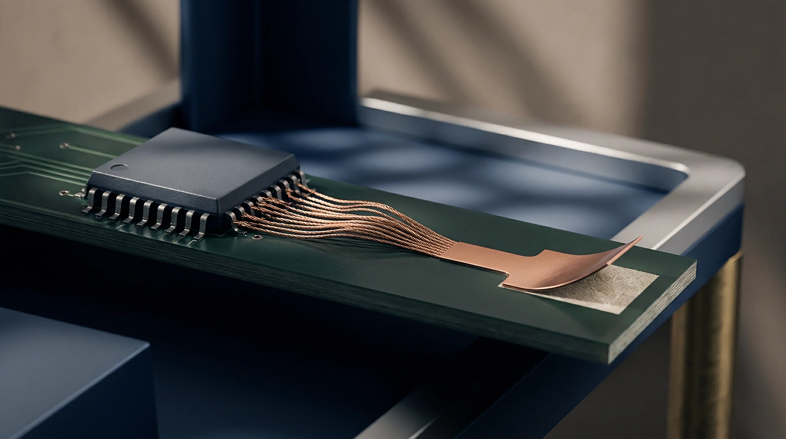
Temperature swings introduce volumetric stress in composite boards, changing resin density while leaving the woven glass frame largely stable. Hydrocarbon polymers exhibit a negative thermal coefficient of dielectric constant, causing relative permittivity to decline as temperature rises. Woven glass fibers, by contrast, possess a slightly positive thermal coefficient and minimal thermal expansion, while ceramic fillers such as silica or metal oxides are added to offset negative resin drift.
Because glass fibers constrain in-plane movement, overall thermal expansion across the substrate becomes strongly anisotropic.
Volumetric thermal expansion is directed almost entirely into the vertical z-axis. Between -40°C and +125°C, z-axis thermal expansion for a high-performance hydrocarbon laminate ranges from 30 ppm/°C to 60 ppm/°C below Tg, whereas in-plane CTE remains bound to the glass weave at 11 ppm/°C to 15 ppm/°C. As temperature increases, vertical matrix expansion reduces resin density along the z-axis. Because z-axis permittivity follows a series capacitive model, this density reduction depresses the vertical dielectric constant far more than in-plane values, shifting the anisotropy ratio across operating temperatures.
Thermal Coefficient of Permittivity Dynamics
Material datasheets often report a single scalar temperature coefficient measured at lower radio frequencies using clamped stripline fixtures. That single number hides how directional permittivity splits over temperature. The temperature coefficient of relative permittivity, Tk varεr, tracks dielectric change per degree Celsius:
Tk varεr = frac1varεr(T0) fracpartial varεr(T)partial T × 106 quad
Evaluated along orthogonal spatial axes, temperature coefficients separate into Tk varεr,z and Tk varεr,xy. Vertical expansion reduces matrix density along the z-axis, making Tk varεr,z substantially more negative than Tk varεr,xy. For a ceramic-filled hydrocarbon laminate with a nominal z-axis dielectric constant of 3.48 at 25°C, the vertical coefficient Tk varεr,z might measure -85 ppm/°C while the in-plane coefficient Tk varεr,xy reads -30 ppm/°C. Over a 100°C temperature rise, z-axis permittivity drops by 0.0296 to 3.4504, whereas in-plane permittivity falls by only 0.0109, shifting the anisotropy ratio from 0.9534 down to 0.9502.
Phase velocity changes as permittivity drifts. Extracting temperature-dependent dielectric drift across standard operating conditions follows a structured test protocol:
- Mount the bare laminate test panel inside a temperature-controlled environmental chamber equipped with low-loss phase-stable coaxial feedthroughs.
- Connect a calibrated vector network analyzer to an integrated substrate cavity resonator designed to excite both TM010 and TE111 modes.
- Establish thermal equilibrium at the lower limit of -40°C, holding the temperature constant for thirty minutes to eliminate internal thermal gradients.
- Record resonant center frequencies and quality factors for both orthogonal field modes at millimeter-wave frequencies.
- Increase chamber temperature in discrete 15°C increments, allowing a twenty-minute soak time at each plateau up to +125°C.
- Calculate isolated z-axis relative permittivity and in-plane relative permittivity at each temperature step using mode-matching field equations.
- Extract directional temperature coefficients Tk varεr,z and Tk varεr,xy by linear regression across the temperature range.
This procedure removes parasitic thermal errors from interconnect cables by de-embedding phase shifts against reference standards placed inside the chamber. Without thermal de-embedding, cable drift degrades substrate measurement accuracy and leads to flawed material selections in early development.

Millimeter Wave Anisotropy Shifts across Operating Temperatures
At 28 GHz and 77 GHz, electromagnetic waves sample microscopic variations in both parallel and perpendicular dielectric constants. As operating frequencies move into millimeter-wave bands, dielectric relaxation in the hydrocarbon polymer alters baseline permittivity. High-frequency relaxation causes resin permittivity to fall smoothly as frequency rises ~ a relationship captured by the Havriliak-Negami dispersion model.
At elevated temperatures, dipolar relaxation frequencies shift closer to the operating band, worsening directional drift.
To see how thermal-anisotropic drift behaves in practice, consider a 77 GHz automotive radar microstrip patch antenna on a 100-micrometer hydrocarbon substrate. At 25°C, nominal z-axis dielectric constant is 3.00 and in-plane dielectric constant is 3.12, giving an initial anisotropy ratio of 0.9615. Patch width W and length L are set to resonate at 77.00 GHz:
L = fracc02 fr sqrtvarεr,eff
Here, c0 is the speed of light in vacuum, fr is resonant frequency, and varεr,eff is the effective dielectric constant derived from z-axis and fringing in-plane permittivity components. Under normal vehicle operation, transmitter heat and solar exposure push board temperature to +105°C ~ an 80°C rise. With a z-axis thermal coefficient Tk varεr,z = -60 p±/°C and in-plane coefficient Tk varεr,xy = -20 p±/°C, permittivity at +105°C shifts to:
varεr,z(105°C) = 3.00 × (1 – 0.0048) = 2.9856
varεr,xy(105°C) = 3.12 × (1 – 0.0016) = 3.1150
The anisotropy ratio drops to 0.9584. That lower effective permittivity speeds up phase velocity, shifting center resonant frequency up by about 185 MHz to 77.185 GHz. In an FMCW radar with a 1 GHz sweep bandwidth, an uncompensated 185 MHz shift creates range errors, raises sidelobe levels, and degrades target detection.
| Laminate Grade | Glass Style | Resin % | varεr,z (10GHz) | varεr,xy (10GHz) | Anisotropy Ratio | Tk varεr,z (ppm/°C) | Tk varεr,xy (ppm/°C) |
|---|---|---|---|---|---|---|---|
| Hydrocarbon/Ceramic A | 106 | 68% | 3.00 | 3.12 | 0.9615 | -50 | -15 |
| Hydrocarbon/Ceramic B | 1080 | 53% | 3.38 | 3.58 | 0.9441 | -75 | -25 |
| Hydrocarbon/Ceramic C | 2116 | 44% | 3.48 | 3.72 | 0.9355 | -110 | -35 |
| Low-Loss Hydrocarbon D | 1035 | 62% | 3.03 | 3.18 | 0.9528 | -40 | -10 |
| Data measured via split-cylinder resonator and cavity perturbation methods per IPC-TM-650 Test Method 2.5.5.13 at room temperature unless noted. | |||||||
Glass fibers keep planar expansion tight. Assuming in-plane dielectric drift follows vertical datasheet values will cause serious phase tracking errors across operating temperatures.
Resonance
Extracting tensor dielectric properties across millimeter-wave frequencies requires fixtures that isolate field components along orthogonal axes. Standard IPC test methods, like clamped stripline fixtures under IPC-TM-650 2.5.5.5, only measure vertical permittivity varεr,z near 10 GHz. These low-frequency scalar numbers say nothing about the anisotropic variation governing lines at 77 GHz or 110 GHz.
At millimeter-wave frequencies, wavelengths drop below 4 millimeters in standard substrates, so parasitic edge radiation, fixture resonance, and surface roughness quickly corrupt measurements.
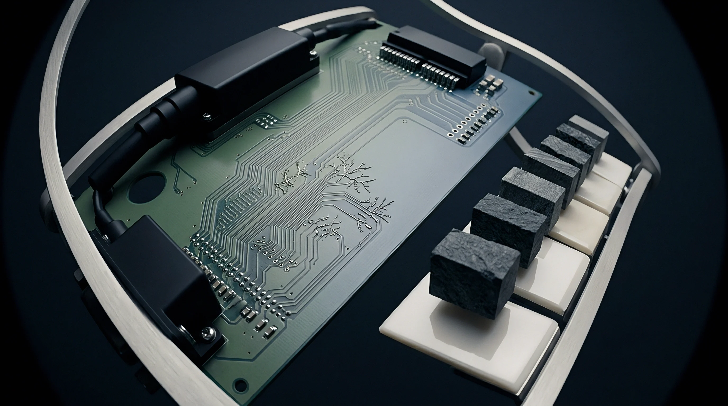
Getting accurate tensor values relies on electromagnetic resonance to decouple out-of-plane fields from in-plane fields. Substrate integrated waveguide (SIW) cavities, split-cylinder resonators, and broadside-coupled ring resonators are the main tools here. By evaluating multiple resonant modes within one cavity, material testing separates varεr,z and varεr,xy over temperature inside environmental chambers.
How Does Cavity Mode Splitting Extract Tensorial Permittivity?
Substrate integrated waveguides and cylindrical metal cavities excite transverse electric and magnetic modes that align with individual material axes. In a circular split-cylinder resonator holding a laminate sample between cavity halves, the fundamental TE011 mode generates electric field lines parallel to the substrate plane. With zero z-axis field component in TE011, measured resonant frequency depends purely on in-plane relative permittivity varεr,xy.
Higher-order transverse magnetic modes like TM010 orient field lines perpendicular to the laminate plane, aligning directly along the z-axis.
Measuring frequency shifts and quality factor degradation across these split modes lets field equations resolve both tensor components independently:
fTE011 = fracc02π sqrtμr varεr,xy sqrtleft(fracx’01aright)2 + left(fracπdright)2
fTM010 = fracc02π sqrtμr varεr,z left(fracx01aright)
In these modal equations, a is cavity radius, d is total cavity height including sample thickness, x01 is the first root of the Bessel function of the first kind, and x’01 is the root of its derivative. Sweeping temperature from -40°C to +125°C inside the cavity tracks frequency shifts in fTE011 and fTM010, giving independent thermal expansion and dielectric drift along each material axis.
Standard factory stripline tests measure only vertical permittivity at 10 GHz, concealing the in-plane dielectric drift that detunes millimeter-wave circuits at elevated temperatures.
Selecting test fixtures for high-frequency qualification comes down to specific trade-offs across measurement tools:
- Split-cylinder resonators isolate in-plane permittivity with high precision but require flat sheet samples with strict thickness uniformity.
- Substrate integrated waveguide cavities allow automated on-wafer probing up to 110 GHz, though copper etching tolerances must be built into the modal model.
- Clamped stripline resonators provide rapid lot-conformance screening at 10 GHz but miss in-plane dielectric parameters completely.
- Ring resonators extract microstrip effective permittivity under actual trace processing conditions, but suffer from radiation loss above 40 GHz.
- Free-space quasi-optical systems eliminate fixture contact errors across broad millimeter-wave bands, but require panels too large for standard temperature chambers.
High-Frequency Fixture Calibration and Fixture De-Embedding
Vector network analyzer measurements above 40 GHz face high parasitic losses from transitions, launch pads, and microstrip-to-coaxial interfaces. These launch parasitics mask the true propagation constant γ = α + jβ of the line. Isolating the phase constant β = ω sqrtμ0 varε0 varεr,eff requires multi-line Thru-Reflect-Line (TRL) calibration standards fabricated directly on the laminate under test.
The TRL protocol uses transmission lines of different electrical lengths to shift the measurement reference plane directly onto the bare substrate line. The phase difference Δ φ between a line of length L1 and a line of length L2 yields the effective relative permittivity:
varεr,eff = left( fracc0 Δ φ2π f (L2 – L1) right)2
Running TRL calibration inside a thermal chamber from -40°C to +125°C isolates the temperature dependence of varεr,eff from cable expansion and connector mismatch drift. Low-frequency factory metrics miss this entirely.
| Test Method Standard | Frequency Range | Primary Field Alignment | Target Permittivity Component | Thermal Chamber Integration | Measurement Uncertainty |
|---|---|---|---|---|---|
| IPC-TM-650 2.5.5.5 Clamped Stripline | 1 GHz – 10 GHz | Out-of-Plane (z-axis) | varεr,z only | Difficult / Poor repeatability | ± 2.0% |
| IPC-TM-650 2.5.5.13 Split-Cylinder | 10 GHz – 40 GHz | In-Plane (x-y plane) | varεr,xy primary | Moderate / Requires thermal insulation | ± 0.8% |
| SIW Cavity Resonance Protocol | 24 GHz – 110 GHz | Dual Mode (TM010 / TE111) | varεr,z and varεr,xy | Excellent / Compact footprint | ± 1.2% |
| Broadside Ring Resonator | 10 GHz – 80 GHz | Fringing / Mixed | varεr,eff (Microstrip) | Good / Standard PCB layout | ± 2.5% |
Using the wrong dielectric extraction method leads to poor material models ~ causing antenna pointing errors, degraded noise figures, and unexpected passband shifts once automotive radar modules are deployed.
Gauge
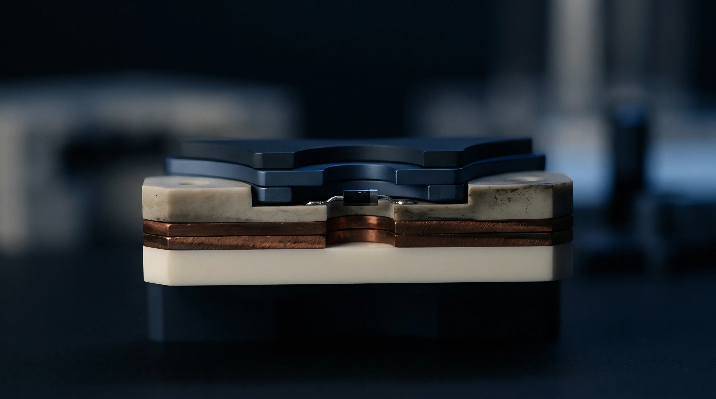
Board shops face immediate challenges turning target dielectric thickness into pressed multilayer stackup specs. Glass-reinforced hydrocarbon laminates behave as visco-elastic solids during pressing cycles. As resin flows, the local ratio of organic binder to glass fabric changes, altering final pressed thickness and anisotropy.
A stackup designed using raw datasheet thickness will miss impedance targets if the shop alters press pressure or prepreg volumes.
Stackup reviews show a 3.8 percent characteristic impedance shift across a 60 Kelvin thermal swing on 77 GHz microstrip lines. That shift came from unexpected compression of 1080 prepreg layers during high-pressure lamination, raising local glass volume fraction and altering vertical dielectric constant. When copper weight, glass weave style, and pressing profile are not aligned, shop-floor tweaks degrade spatial dielectric uniformity.
Resin Content and Prepreg Style Selection
Matching dielectric layer thickness to target impedance constraints requires balancing glass style against press pressure. Prepregs used in hydrocarbon builds consist of woven glass impregnated with uncured or B-stage resin. During lamination, press temperature passes the resin softening point, letting liquid polymer flow and fill voids between etched inner-layer copper traces.
Excessive resin squeeze-out increases glass volume fraction in the cured board, shifting permittivity toward the higher glass value. Because lamination pressure changes glass fill fraction, fabrication notes often call for high-resin prepregs ~ like style 106 (68% resin) or style 1035 (62% resin) ~ paired with low-flow press cycles. Lighter glass styles minimize E-glass yarn mass, narrowing the spread between parallel and series capacitive behavior.
To keep compression and dielectric tolerances tight during lamination, fabricators follow specific pressing steps during inner-layer processing:
- Pre-bake core laminates at 120°C for two hours prior to inner-layer photoimaging to evacuate absorbed moisture and relieve mechanical stress.
- Apply vacuum below 15 mbar inside the press chamber before initiating heat cycles to prevent micro-voids in ceramic filler pockets.
- Ramp press temperature at 2.5°C/min to 3.5°C/min to synchronize resin viscosity drop with vacuum degassing.
- Hold peak lamination pressure at 250 psi for seventy-five minutes at 185°C to cross-link the polymer fully without causing excessive resin squeeze-out.
- Cool the pressed panel under full pressure at no more than 2.0°C/min to minimize built-in stress and z-axis CTE distortion.
Failing to control cooling ramp rates leaves residual stress at the resin-glass interface, worsening dielectric drift during thermal cycling.
Copper Profile Roughness and Skin Depth Interactions
At 77 GHz, current flows through a skin depth under 0.25 micrometers, making micro-topography critical to wave speed. Copper foil treatments added to bond resin create tooth profiles from 1.0 to 3.5 micrometers in peak-to-valley height (Rz). At millimeter-wave frequencies, electromagnetic waves follow these copper contours, extending effective electrical length and slowing phase velocity.
This phase retardation acts like an artificial rise in substrate dielectric constant, referred to as effective rough-copper permittivity varεr,rough. The interaction is modeled with Hammerstad-Bekkadal or modified Cannon roughness equations:
varεr,rough = varεr,smooth left( 1 + frac2π arctan left( 1.4 left 2 right) right)
In this relationship, Rq is root-mean-square surface roughness, δ is skin depth, and varεr,smooth is bare laminate dielectric constant. Since foil treatments sit on horizontal copper sheets, their capacitive impact hits z-axis field lines in microstrips hardest. Standard electrodeposited (ED) copper with Rq of 1.8 micrometers increases effective z-axis dielectric constant by up to 12 percent at 77 GHz, whereas Hyper-Very-Low-Profile (HVLP) copper with Rq of 0.4 micrometers keeps that shift under 2 percent.
| Layer Position | Material Type | Nominal Thickness | Glass Style | Pressed varεr,z (77GHz) | Pressed varεr,xy (77GHz) | Effective Rough varεr |
|---|---|---|---|---|---|---|
| L1-L2 Dielectric | Hydrocarbon Prepreg | 100 $mu$m | 106 (1 ply) | 3.02 ± 0.04 | 3.14 ± 0.05 | 3.10 (HVLP Foil) |
| L2-L3 Core | Hydrocarbon Core | 250 $mu$m | 2116 (1 ply) | 3.48 ± 0.05 | 3.71 ± 0.06 | 3.62 (VLP Foil) |
| L3-L4 Dielectric | Hydrocarbon Prepreg | 150 $mu$m | 1080 (1 ply) | 3.38 ± 0.04 | 3.56 ± 0.05 | 3.50 (VLP Foil) |
| L4-L5 Core | Hydrocarbon Core | 250 $mu$m | 2116 (1 ply) | 3.48 ± 0.05 | 3.71 ± 0.06 | 3.62 (VLP Foil) |
| L5-L6 Dielectric | Hydrocarbon Prepreg | 100 $mu$m | 106 (1 ply) | 3.02 ± 0.04 | 3.14 ± 0.05 | 3.10 (HVLP Foil) |
Hyper-Very-Low-Profile copper foils with surface roughness below 0.5 micrometers eliminate phase velocity retardation caused by rough tooth profiles at 77 GHz.
When releasing mmWave stackups to production, fabricators often substitute equivalent prepreg grades or copper profiles to reduce material costs. Slash-sheet equivalent laminates match nominal 10 GHz dielectric constants on datasheets, but differences in anisotropy and surface roughness alter 77 GHz line impedance and thermal phase drift.
Allowance
Commercial high-frequency board procurement often stumbles because purchase specs rely on low-frequency material callouts. Millimeter-wave boards demand specs covering raw material slash sheets, physical construction, glass weave style, copper treatment, and thermal dielectric drift limits. When purchasing documents skip anisotropy controls or thermal drift bounds, shops tend to pick cheaper heavy-glass alternatives that meet nominal thickness but push phase performance out of spec.
Buying bare panels by area means accounting for panel utilization. Hydrocarbon laminates cost six to ten times more per panel than high-Tg FR-4. Standard production panel sizes are 18 by 24 inches (457 by 610 mm) or 16 by 18 inches (406 by 457 mm).
Unusable borders for conveyor rails, tooling targets, test coupons, and plating clamps eat up to 25 percent of gross panel area. If PCB dimensions don’t nest cleanly inside the active area, unit costs climb fast.
Commercial Procurement and Panel Yield Optimization
Purchasing agents calculate board costs from usable square area on standard 18 by 24 inch panels. Efficient layouts maximize working circuits per sheet while leaving room for scoring and routing tools. When drawing notes specify tight dielectric thickness tolerances (± 5% instead of standard ± 10%), fabricators lower yield estimates and pad unit prices with higher scrap allowances.
To establish clear technical constraints on purchase orders, RFQ packages should include specific fabrication notes that lock down material properties without driving up yield scrap:
- Material qualification notes mandate specific hydrocarbon laminates by product series rather than generic IPC slash sheets.
- Reinforcement fabric notes lock allowable glass styles on signal layers to stop shops from swapping light fabric for heavy weaves.
- Copper foil specifications define maximum surface roughness Rq on signal layers and mandate HVLP treatment.
- Thermal drift limits set the maximum change in effective dielectric constant across -40°C to +125°C.
- Coupons and test requirements mandate TRL calibration and resonance structures on panel margins for lot acceptance testing.
Specifying z-axis dielectric constant tolerances at 10 GHz and 77 GHz separately on fabrication drawings prevents vendor misinterpretation. When procurement dockets specify core materials and prepreg press profiles, shops maintain consistent line impedance across production lots.
Fabrication Notes and Quality Verification Standards
Engineering drawings act as legal specs governing material substitution and quality assurance. Industry performance specs like IPC-6012 Class 3 or Class 3/A dictate strict controls for annular rings, plating thickness, and voiding, but they say nothing about high-frequency dielectric anisotropy or thermal phase shift limits. Supplemental drawing notes bridge that gap by setting enforceable electrical standards.
When drafting release notes for millimeter-wave hydrocarbon panels, drawing notes should establish explicit electrical acceptance criteria tied to lot delivery:
Fabrication note specification line: “Controlled impedance transmission lines on Layer 1 and Layer 6 shall be verified using on-panel TRL coupon structures measured at 77 GHz ± 2 GHz. The effective dielectric constant derived from coupon phase measurements shall not vary by more than ± 1.5% across the operating thermal range of -40°C to +125°C, and total anisotropy ratio (varεr,z / varεr,xy) shall remain within 0.940 to 0.965. Deliveries failing coupon phase tracking criteria shall be subject to lot rejection at the supplier’s expense.”