Mapping High Speed Power Grid Transfer Impedance to Emissions Limits
Mapping high-speed power rail transfer impedance limits directly to radiated emissions limits prevents costly EMC chamber re-tests and batch rejections.
Plane

Dynamic Current Injection and Common Mode Conversion
A high-speed power distribution network behaves like a distributed reactive circuit rather than a clean zero-impedance rail. As integrated circuits pull transient switching currents with nanosecond edge rates, they trigger structural resonances between internal power and ground plane pairs. Transfer impedance ~ the complex ratio of induced voltage at an outlying point to injection current at the die pad ~ determines how effectively that local noise spreads across the board.
High transfer impedance peaks turn localized current steps into board-wide voltage ripple, driving common-mode currents straight into chassis structures, peripheral cables, and board edges.
At frequencies where board dimensions approach the dielectric wavelength, the plane pair turns into a cavity resonator. If dynamic switching harmonics hit one of these structural modes, transfer impedance can spike ten- to a hundred-fold over the low-frequency target impedance. These resonances build sharp voltage peaks along apertures and perimeter edges.
Fringing fields at unshielded board boundaries then leak across outer dielectric layers, converting differential rail noise into radiated electric fields.
Edge radiation from resonant planes remains a primary failure mode during compliance testing of dense digital layouts. Common-mode voltage turns connected I/O lines into efficient dipole or monopole radiators. At five hundred megahertz, an unmitigated transfer impedance peak needs less than ten microamperes of common-mode current to blow through standard commercial limits at three meters.
Tackling these issues with chassis shielding after layout locks in extra unit cost and compromises delivery schedules.
Overlooking transfer impedance during layout leaves field failures that supplemental shielding cannot reliably cure.
Ripple
Cavity Resonance and Parasitic Inductance
Power plane antiresonance develops when the capacitive reactance of a plane pair or capacitor array balances the inductive reactance of component mounting loops and package parasitics. While thin plane spacing yields low impedance well into the high frequencies, discrete decoupling capacitors introduce both equivalent series inductance and mounting loop inductance. Above the array self-resonant frequency, this loop inductance dominates, driving transfer impedance up at twenty decibels per decade until it meets the plane capacitance resonance.
Observed transfer impedance varies considerably by physical location on the printed circuit board. Two-dimensional wave equations predict where these cavity peaks will land based on plane geometry, dielectric properties, and boundary conditions:
f_mn = (c / (2 pi sqrt(er))) sqrt((m pi / a)^2 + (n pi / b)^2)
where a and b represent plane length and width, er is the relative dielectric permittivity, c is the speed of light in vacuum, and m, n represent structural mode numbers. At mode frequencies, impedance collapses near voltage nodes but climbs steeply at anti-nodes, which makes single-value target impedance calculations unreliable for estimating high-frequency emissions.
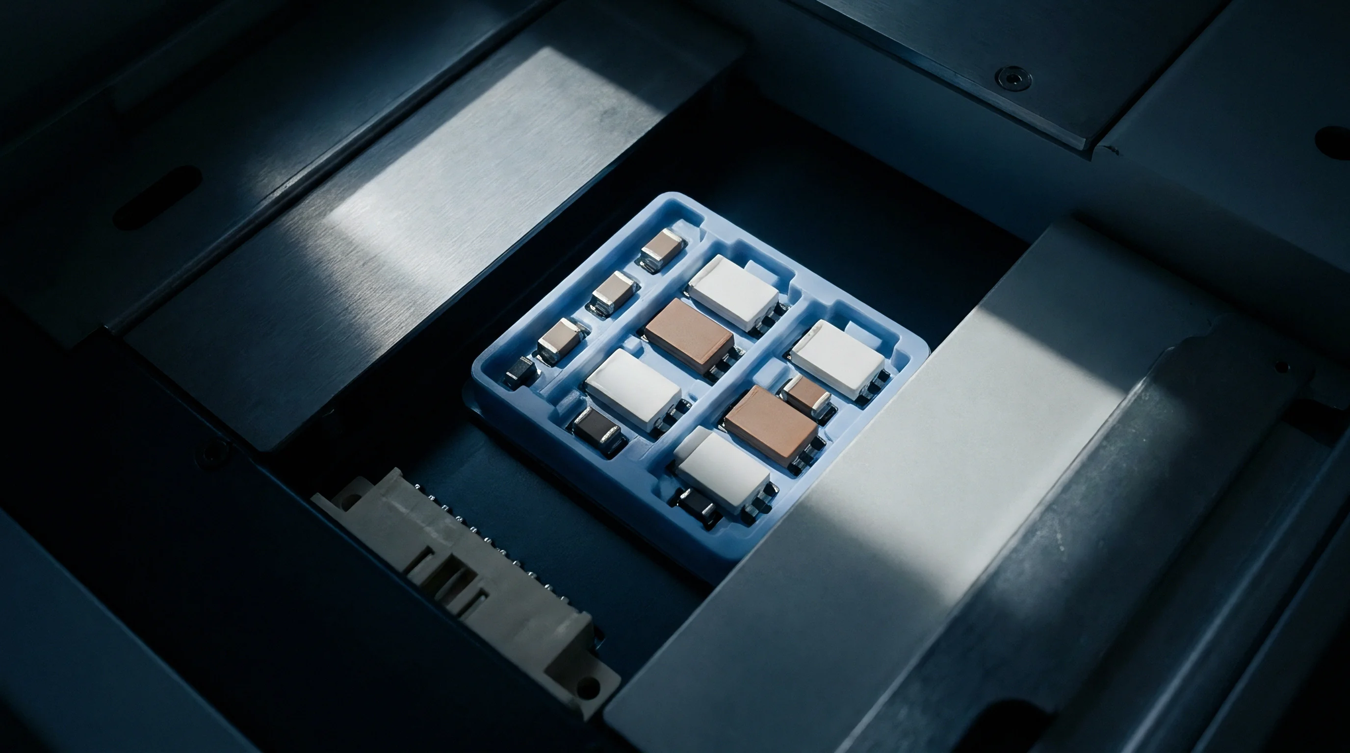
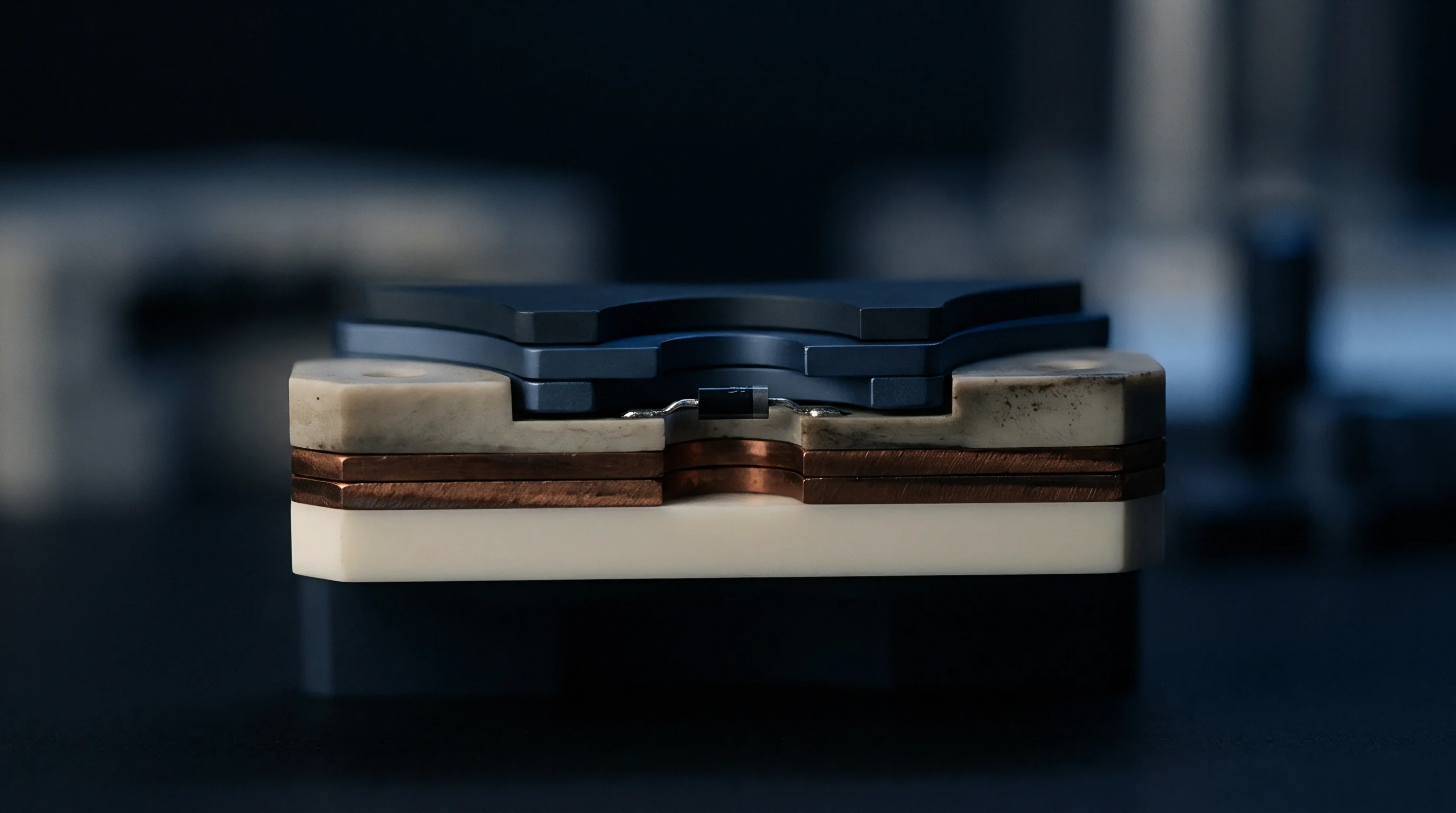
Operational heating and DC bias shift these decoupling networks over time. High-permittivity ceramic capacitors lose significant effective capacitance under DC voltage, shifting array resonance up into the paths of active switching harmonics. Thermal cycling also fractures ceramic terminations, pushing up equivalent series resistance and dulling high-frequency bypass response.
These shifting peaks reshape the radiated profile, so a board passing comfortably at room temperature can fail once fully loaded in the field.
The table below shows measured antiresonant peak drift and loop inductance growth caused by dielectric aging under temperature and DC bias voltage stress.
| Dielectric Class | Applied DC Bias Ratio | Temperature Shift | Nominal Capacitance Retention | Antiresonant Peak Frequency Shift | Impedance Magnitude Increase at 400 MHz |
|---|---|---|---|---|---|
| X7R High Permittivity | 0 Percent | 25 Degrees Celsius | 100 Percent | Baseline (320 MHz) | 0.0 dB |
| X7R High Permittivity | 50 Percent Nominal | 65 Degrees Celsius | 68 Percent | +18 Percent (378 MHz) | +4.2 dB |
| X7R High Permittivity | 80 Percent Nominal | 85 Degrees Celsius | 42 Percent | +39 Percent (445 MHz) | +8.5 dB |
| X5R Ultra Compact | 80 Percent Nominal | 85 Degrees Celsius | 29 Percent | +58 Percent (505 MHz) | +12.1 dB |
Capacitor mounting loop inductance dictates high-frequency impedance limits long before board-level plane capacitance takes effect.
Suppression Strategies for Board Level Resonances
Damping transfer impedance peaks takes careful capacitor placement, tight loop inductance control, and deliberate plane shaping. Scattering more decoupling capacitors across the board without planning often introduces new antiresonant spikes that merely push emissions into another band.
- Capacitor Mounting Optimization drops loop inductance by dropping via pairs right against component pads and keeping surface traces short and wide.
- Edge Via Shielding Arrays form perimeter Faraday walls that terminate lateral cavity modes and drop edge-radiated field levels by up to fifteen decibels.
- Interplane Dielectric Thinning raises structural capacitance, pushing cavity resonances above critical clock harmonics while flattening impedance peaks.
- Lossy Ferrite Integration burns off high-frequency energy at known anti-nodes without degrading DC supply performance.
High-frequency impedance control works only when component layout targets physical cavity modes instead of gross microfarad totals.

Scan
Measurement Regimes for Transfer Impedance Verification
Mapping transfer impedance across high-speed rails demands vector network analyzer setups resolved down into the milliohm range. Conventional two-port S-parameter sweeps create ground loop paths that swamp readings below one ohm. Using two-port shunt-thru methods with coaxial common-mode chokes or isolation transformers cuts these ground loops, giving clean data down into the milliohm range up to three gigahertz.
Micro-coaxial probes calibrated right at the tips through Short-Open-Load-Through standards strip out fixture inductance and cable loss before data collection. Calibration transfer errors distort measured antiresonance heights, hiding peaks that drive field failures. De-embedding routines strip out pad parasitics to isolate the bare transfer impedance matrix between die injection points and perimeter nodes.
Plotting two-port S21 transfer sweeps alongside radiated emissions data from a Semi-Anechoic Chamber ties bench metrics directly to test chamber performance. Transfer impedance peaks track electric field spikes captured during ten-meter antenna sweeps with remarkable consistency. Spotting these rail peaks on the bench catches layout flaws well before full qualification runs.
A transfer impedance spike of two hundred milliohms at six hundred megahertz drives a four-microampere common-mode current that exhausts CISPR 32 Class B margins.
Several setup errors distort transfer impedance traces, producing false margins during bench reviews:
- Uncompensated Cable Loop Currents add series resistance that masks resonance dips and hides true transfer impedance peaks.
- Probe Tip Contact Resistance Variances alter measured Q factors, making dangerous antiresonances look damped and harmless on the screen.
- Inadequate VNA Dynamic Range masks baseline plane performance beneath instrument noise, skewing calculated decoupling needs.
- Calibration Drift Under Ambient Temperature Swings skews phase measurements, invalidating de-embedding math past one gigahertz.
Radiated failures above several hundred megahertz frequently trace to internal board impedance peaks rather than harness coupling.
Bound
Converting Transfer Impedance to Radiated Field Strength
Direct analytical relationships link power grid transfer impedance to the radiated limits in CISPR 32 and FCC Part 15. The core structure models the plane pair and attached traces as an antenna driven by switching currents at the silicon. At a specified distance, the radiated field scales with current draw, transfer impedance, and a structural antenna factor:
E(f) = k f Z_21(f) I_die(f) AF(f)
where E(f) is electric field strength in volts per meter, f is frequency, Z_21(f) is transfer impedance, I_die(f) is the dynamic switching spectrum, AF(f) is the structural antenna factor of the assembly, and k captures geometry and propagation constants.

Where Does Transfer Impedance Exceed Permissible Emissions Thresholds?
Setting an upper boundary for allowable transfer impedance requires defining maximum rail transients and structural radiation efficiency. Take an application processor on a 1.2V core rail drawing 4A transients at 250 MHz, with harmonic energy reaching 1.25 GHz. Assume an antenna factor of 0.02 m^-1 at 750 MHz across the board edge and harness, tested at 3 meters against CISPR 32 Class B (40 dBµV/m, or 100 µV/m).
At the 750 MHz third harmonic, dynamic switching current reaches roughly 0.8A. Calculating the target transfer impedance Z21(f) with a 6 dB safety margin (holding field strength to 50 µV/m):
Z_21_max = E_limit / (k f I_harmonic AF)
Plugging in these operating terms sets the ceiling. At 750 MHz, transfer impedance cannot exceed 62 milliohms without crossing the emission threshold.
| Harmonic Frequency | Dynamic Current (A) | Transfer Impedance (mΩ) | Antenna Factor (m⁻¹) | Calculated Field at 3m (dBµV/m) | CISPR 32 Class B Limit (dBµV/m) |
|---|---|---|---|---|---|
| 250 MHz | 2.40 | 120 | 0.005 | 31.2 | 40.0 |
| 500 MHz | 1.20 | 180 | 0.012 | 38.4 | 40.0 |
| 750 MHz | 0.80 | 240 | 0.020 | 45.8 | 40.0 |
| 1000 MHz | 0.45 | 310 | 0.035 | 48.1 | 47.0 |
EN 55032 Clause 10 mandates strict limits on radiated field strengths, making pre-test board-level impedance limits a primary acceptance gate for imported electronics.
Specifying a maximum transfer impedance in production contracts requires fabrication plants to hold tight tolerances on plane spacing and component placement across incoming lots.
Forfeit
Lot Variance and Conformity File Obligations
Component and manufacturing variations cause measurable shifts in transfer impedance throughout volume assembly. Changes in prepreg dielectric thickness, voiding under decoupling solder pads, or layer misalignment in ceramic capacitors all move local impedance peaks. As a result, a design that sails through qualification on engineering prototypes can trigger regulatory rejections once volume variations slide those peaks onto active clock lines.
Technical construction files under EN IEC 63000 require proof of control over any production change that influences electromagnetic performance. Changing a capacitor manufacturer, laminate source, or inner copper weight alters the distribution network impedance profile. Manufacturers and importers signing CE declarations bear direct liability for production conformity; a test certificate from an early prototype provides zero legal protection if material changes pushed a volume run out of compliance.
The protocol below outlines the verification steps required before releasing volume shipments:
- Perform two-port VNA shunt-thru impedance sweeps across all high-speed power rails on five sample boards per production batch.
- Compare extracted antiresonant peak amplitudes and frequencies against maximum allowable transfer impedance limits derived during initial qualification.
- Reject any manufacturing lot exhibiting a transfer impedance increase exceeding three decibels at critical clock harmonic frequencies.
- Verify decoupling capacitor ceramic dielectric lot numbers against approved bill-of-materials specifications to prevent unapproved DC bias voltage degradation.
- Archive calibrated S-parameter files alongside thermal scan records within the mandatory technical construction file for ten years post-market release.
Non-compliant production batches detained at customs borders impose storage costs and logistics penalties that exceed original design budgets.
How far must an importer extend batch-level impedance verification before component tolerance shifts render historical EMC test reports legally invalid?