Understanding Directional Dielectric Permittivity Variance in Multilayer Stackups
Multilayer directional permittivity variance causes stripline capacitance shifts that must be corrected by modeling in-plane and out-of-plane dielectric constants separately.

Resin
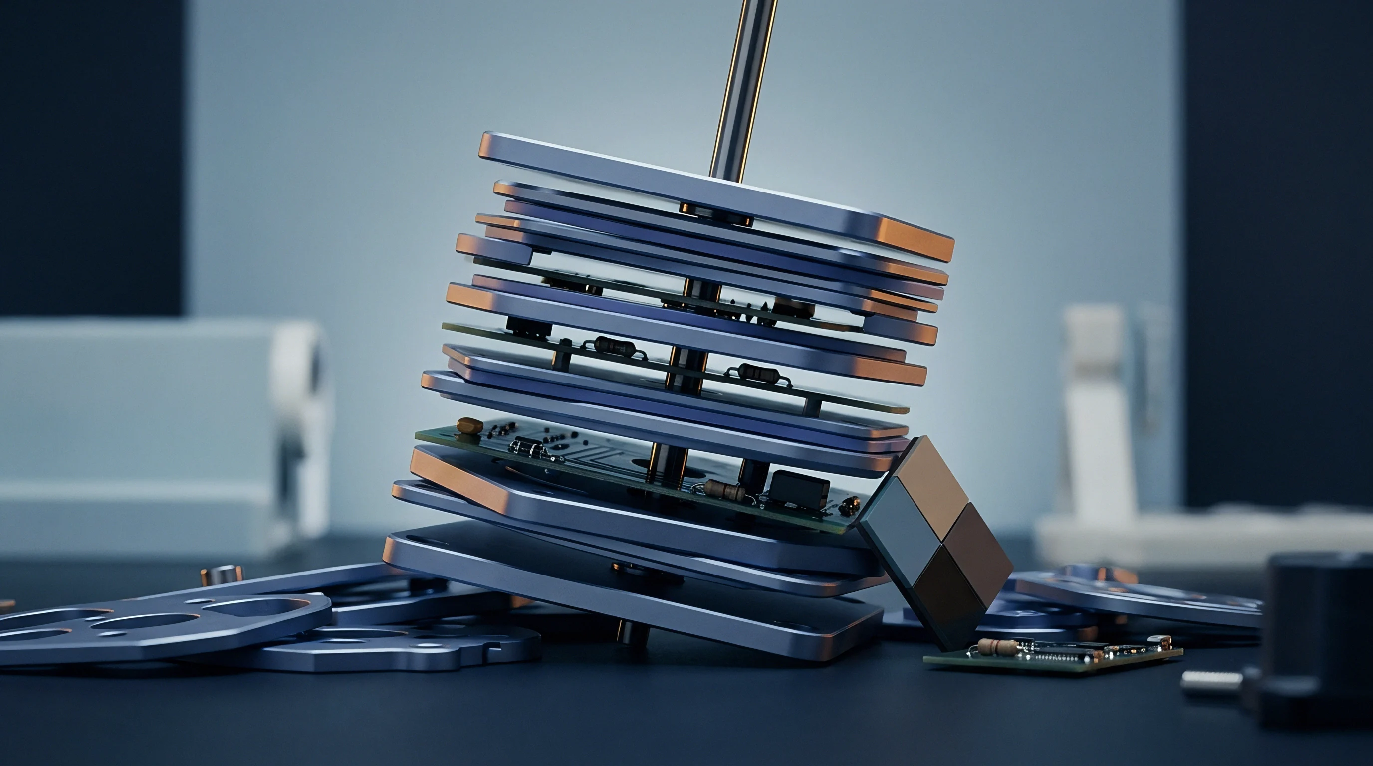
Multilayer circuit boards are built on composite dielectrics where synthetic polymer matrices bind woven glass cloth. When electric fields propagate through these structures, they interact with two materials that have drastically different electrical properties. E-glass reinforcement exhibits a relative dielectric constant between 6.1 and 6.6 at microwave frequencies, while thermosetting resin systems typically sit between 2.8 and 3.4.
The spatial distribution of these components creates anisotropic dielectric behavior across the board’s three principal axes. As a result, the dielectric constant measured perpendicular to the laminate plane (the out-of-plane or z-axis permittivity) often differs by 5 to 15 percent from the value measured parallel to it (the in-plane or xy-axis permittivity).
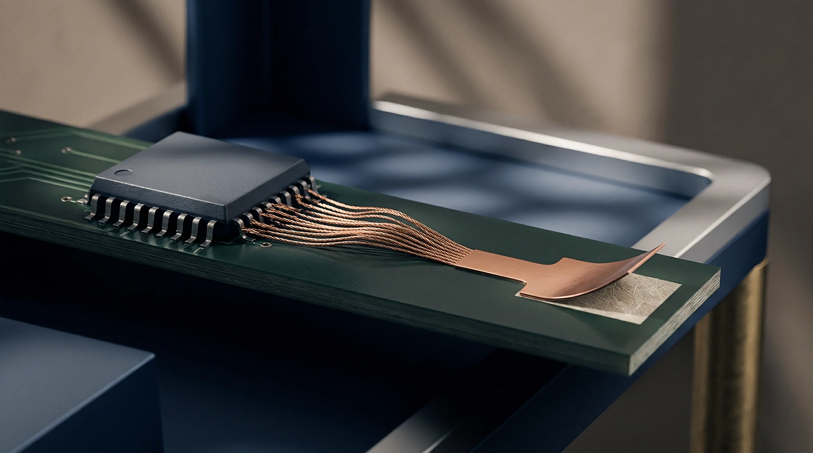
This anisotropy invalidates simple isotropic modeling. Circuit designers who rely on the single dielectric constant listed on a laminate datasheet frequently run into timing shifts and impedance mismatches when traces transition between microstrip and stripline layers. In microstrip routing, fields extend outward from the trace through solder mask, air, surface resin, and the underlying glass fabric.
Stripline geometries keep the fields inside the substrate core, directing primary flux along the z-axis while fringing fields extend laterally through the xy-plane. Because flux distribution changes with trace topology, the effective permittivity depends directly on conductor orientation relative to the composite microstructure.
Molecular Orientation and Out-of-Plane Electric Fields
Polymer chains in thermosetting matrices align during high-temperature curing under hydraulic press pressure. Cross-linked epoxy, polyphenylene ether, and polyimide matrices compress vertically while the resin is fluid, flattening polymer backbones into planar orientations parallel to the foil boundaries. Electric field vectors oriented along the z-axis perpendicular to these chains encounter different polarizability than fields running parallel to the backbones.
This orientation depresses out-of-plane permittivity compared to unaligned, isotropic cured resins.
Orthogonal trace runs sharing identical nominal dimensions on multi-layer backplanes can show up to a 7.2 percent impedance discrepancy. Vertical flux lines have to cross alternating planar layers of pure resin and dense glass filaments. The series capacitive combination of high-permittivity glass and low-permittivity resin lowers the effective capacitance per unit length along the z-axis.
Conversely, lateral fields running parallel to the reinforcement layers pass through continuous regions of glass and resin simultaneously, acting as parallel capacitive networks dominated by the higher-permittivity glass phase and driving up in-plane Dk.
Under IPC-TM-650 Method 2.5.5.5 testing at 10 GHz, a 55 percent resin content prepreg yields an out-of-plane dielectric constant of 3.62 against an in-plane value of 3.98.
Resin Content Impact on Bulk Anisotropy Ratios
Standard prepreg styles use different resin-to-glass ratios to achieve specific pressed thicknesses. High-resin weaves like 106 and 1080 have resin volume fractions exceeding 65 percent, whereas heavy styles like 7628 stay below 45 percent. Substrates with high resin volume fractions push the anisotropic permittivity ratio closer to unity because the isotropic polymer phase dominates the bulk volume.
Low-resin laminates elevate bulk permittivity while widening the gap between in-plane and out-of-plane dielectric constants.
The anisotropy ratio scales directly with this resin fraction. When high-speed digital signals travel along microstrip traces on low-resin dielectrics, lateral fringing capacitance encounters an effective dielectric constant significantly higher than the z-axis baseline assumed by automated field solvers. Calculating signal propagation delay from published z-axis datasheet values understates true line delay by up to 4.5 picoseconds per inch on 7628-based multilayer stackups.
Because field lines penetrate epoxy and glass unevenly, out-of-plane fields see a lower average permittivity across the stackup. Resin completely fills the inter-yarn gaps, and the resulting glass-to-resin balance sets the baseline physical geometry through which all electrodynamic fields propagate ~ creating structural variances that test equipment and design rules must account for.
What remaining thermodynamic factors during lamination pressure cycles alter resin polymer chain orientation across high-layer-count backplane panels?
Fiber
Woven glass fabric provides the mechanical framework for rigid multilayer printed circuit boards. Continuous filaments of E-glass or low-loss NE-glass are bundled into yarns, which automated looms weave into grid patterns defined by warp and fill orientations. Warp yarns run continuously along the length of the roll under high mechanical tension.
Fill yarns run across the roll width under noticeably lower tension. This mechanical imbalance results in asymmetric bundle flattening, spacing, and glass distribution along the panel’s orthogonal axes.
That structural asymmetry produces periodic dielectric variation across the board surface. Common glass styles like 106, 1080, 2116, and 7628 feature distinct warp and fill yarn counts. A 1080 fabric, for instance, has 60 warp yarns and 47 fill yarns per inch, leaving open resin-rich window spaces between bundle intersections.
Traces routed directly over yarn bundles see a local dielectric constant dominated by glass, while traces over open windows see permittivity governed primarily by the resin matrix.
Glass Fabric Style Selection and Yarn Spacing
Yarn geometry dictates the severity of localized dielectric fluctuations across the board. Conventional weaves leave open rectangular windows where resin pools during lamination. Mechanically spread-glass fabrics ~ such as 1035, 1078, and 3313 ~ flatten yarn bundles into wide ribbons during production.
This spreading minimizes resin windows, producing a continuous glass sheet with far more uniform local permittivity.
Heavier glass weaves introduce much wider dielectric variations. Standard 7628 fabric uses coarse yarn bundles that yield thick layers at the expense of localized Dk swings up to 0.40 units between bundle centers and window centers. Spread-glass styles pull this ripple below 0.05 units.
Specifying spread-glass laminates prevents differential phase skew by ensuring both lines in a high-speed differential pair experience identical effective permittivity along their route.
| Glass Style | Yarn Count (Warp × Fill per inch) | Nominal Pressed Thickness (mm) | Resin Content (%) | Out-of-Plane Dk (z-axis) | In-Plane Dk (xy-axis) | Anisotropy Ratio (Dk_xy / Dk_z) |
|---|---|---|---|---|---|---|
| 106 | 56 × 56 | 0.033 | 72 | 3.45 | 3.72 | 1.078 |
| 1078 (Spread) | 54 × 54 | 0.041 | 64 | 3.58 | 3.88 | 1.084 |
| 1080 | 60 × 47 | 0.064 | 65 | 3.60 | 3.91 | 1.086 |
| 2116 | 60 × 58 | 0.094 | 54 | 3.78 | 4.14 | 1.095 |
| 3313 (Spread) | 61 × 62 | 0.084 | 57 | 3.72 | 4.05 | 1.089 |
| 7628 | 44 × 31 | 0.173 | 43 | 4.10 | 4.55 | 1.110 |
| Data compiled per IPC-TM-650 Method 2.5.5.5 (clamped stripline) and SPDR test methods at 23°C ambient. | ||||||
Warp and Fill Direction Permittivity Divergence
Unequal yarn densities between warp and fill axes create in-plane dielectric anisotropy (Dkx ≠ Dky). In 7628 glass, 44 warp yarns per inch pack tightly together, while 31 fill yarns per inch leave larger resin gaps. Signal lines routed parallel to the warp axis encounter a higher volumetric ratio of glass per unit length than lines running parallel to the fill axis.
This directional disparity shifts characteristic impedance and propagation velocity between traces routed 90 degrees apart on the same layer.
Routing critical high-speed tracks diagonally across the fabric grid resolves this warp/fill divergence. Off-axis routing forces traces to cross both yarn directions at consistent 45-degree angles, averaging out glass volume variations over short distances. PCB fabricators can implement this by rotating artwork files relative to the panel boundary or shifting panel orientation during raw sheet cutting, though panel rotation reduces raw material yield.
Aligning high-speed signal tracks off-axis relative to the laminate weave eliminates glass-weave trace skew without changing material suppliers.
Glass fibers dictate the in-plane dielectric response. Because dimensional stability during pressing depends on yarn tension control during weaving, the way resin fills interstitial gaps under heat and pressure ultimately determines how dielectric variation is distributed across the finished board.


Resonator
Extracting accurate dielectric properties from unclad laminates requires test fixtures whose boundary conditions align with specific field orientations. Material vendors select characterization methods designed for quality control rather than predictive modeling. Standard datasheets publish permittivity derived from IPC-TM-650 methods intended for lot-to-lot screening, but these fixtures typically isolate a single axis and mask directional variations present in finished multilayer boards.
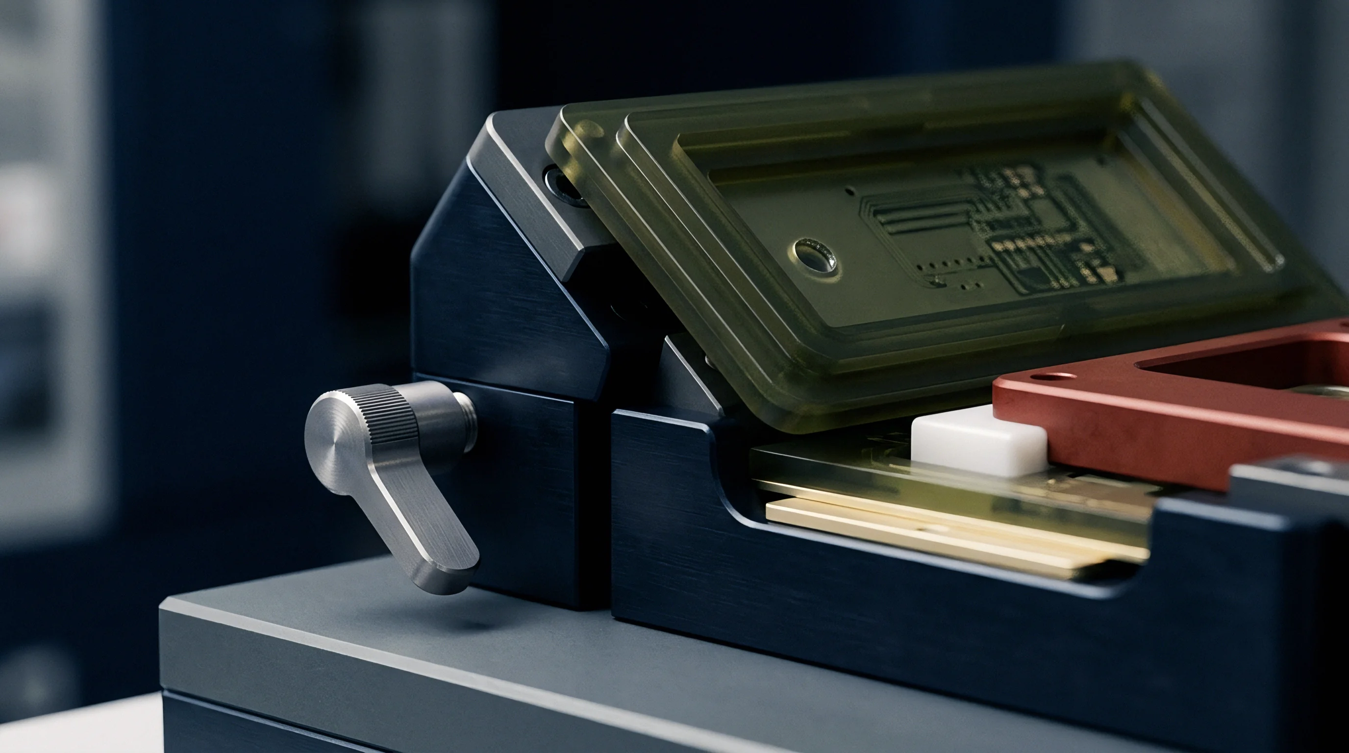
The fixture chosen determines which tensor component is measured. Clamped stripline fixtures measure out-of-plane permittivity by compressing unclad dielectric sheets between ground planes, applying normal force to squeeze out air gaps. Split-post dielectric resonators evaluate in-plane properties by placing substrates inside a resonant cavity where electric field vectors lie parallel to the sample sheet.
Side-by-side comparison of data from both fixtures reveals the full extent of anisotropy in composite laminates.

Standardized Test Method Discrepancies across Axis Orientations
IPC-TM-650 Method 2.5.5.5 relies on a clamped stripline fixture operating between 8 GHz and 10 GHz. The electric field runs strictly perpendicular to the sample, measuring only the z-axis relative dielectric constant (Dkz). Air gaps between the fixture plates and unclad dielectric samples reduce measured capacitance, requiring high clamping pressures or fluid immersion to correct readings.
Crucially, this method ignores lateral electric field components, masking the higher in-plane permittivity seen by actual signal traces.
Split-post dielectric resonator (SPDR) fixtures test sheets by exciting TE011 mode microwave fields inside a high-Q cavity. Fields circulate parallel to the test specimen, measuring purely in-plane permittivity (Dkxy). SPDR measurements consistently yield permittivity values 6 to 12 percent higher than IPC-TM-650 Method 2.5.5.5 tests on identical material lots.
When field solvers are configured solely with clamped stripline data, they inevitably underestimate physical microstrip capacitance.
Why Do Datasheet Dielectric Values Fail in Field Calculations?
2D field solvers rely on single scalar dielectric constants when solving Maxwell’s equations for trace capacitance and inductance. If a designer inputs a datasheet value measured via z-axis clamped stripline, the solver assumes the material is isotropic. In a microstrip trace, however, up to 40 percent of the total flux spreads laterally through the board along the in-plane axis.
Using an out-of-plane Dk of 3.60 for a core with an in-plane Dk of 3.95 forces the solver to undercalculate capacitance, resulting in fabricated trace impedances 2 to 4 ohms higher than intended.
Substrate suppliers publish out-of-plane permittivity values. Measurement fixtures alter field distribution patterns. Evaluating raw substrate vendors requires auditing coupon test reports against microsection data.
Using unadjusted datasheet dielectric constants for stripline design introduces subtle timing discrepancies. In stripline traces, while primary fields align along the z-axis, fringing fields at conductor edges propagate laterally through the higher-permittivity xy-plane. Conductor edge thickness, controlled by copper foil weight, dictates the proportion of fringing field flux passing through the in-plane dielectric zone.
A practical example illustrates the severity of anisotropic modeling errors. Consider a 50-ohm single-ended stripline on a 0.100 mm dielectric layer using 1-ounce copper (0.035 mm thick conductor). Standard IPC-TM-650 2.5.5.5 data specifies a z-axis dielectric constant (Dkz) of 3.70 at 10 GHz.
An isotropic field solver using Dk = 3.70 calculates a required trace width of 0.122 mm to hit 50.0 ohms impedance.
Modeling the same trace with tensor anisotropic permittivity gives a very different picture. SPDR testing on the same material lot shows an in-plane dielectric constant (Dkxy) of 4.10. An anisotropic field solver accounts for the 0.035 mm conductor sidewalls, where lateral fringing fields travel through the Dkxy = 4.10 medium while vertical flux sees Dkz = 3.70.
The effective dielectric constant experienced by the signal climbs to 3.82.
Under isotropic assumptions, the 0.122 mm trace actually produces a characteristic impedance of 48.3 ohms ~ a 1.7-ohm shortfall that can blow tight system budgets. Hitting a true 50.0-ohm transmission line requires narrowing the trace to 0.115 mm. Signal velocity drops accordingly, pushing propagation delay from 152.3 picoseconds per inch up to 154.8 picoseconds per inch.
On synchronous 28 Gbps parallel buses, a 2.5 picosecond per inch timing discrepancy consumes a large portion of the allowable window.
- Clamped Stripline Fixtures measure z-axis permittivity under high normal force, ignoring lateral fringing field interactions and omitting copper foil surface roughness contributions.
- Split-Post Resonators isolate in-plane permittivity without contacting conductor metallization, operating accurately only on thin, unclad dielectric sheet samples.
- Full-Sheet Resonators evaluate total panel capacitance at low radio frequencies, averaging spatial variances while failing to capture high-frequency dispersion dynamics.
- Ring Resonator Coupons extract effective dielectric constants from etched circuit traces, incorporating production etch factors and copper roughness while confounding material anisotropy with geometric etching variances.
High-density interconnector builds risk failing characteristic impedance qualification when field solvers rely on clamped stripline datasheet values rather than tensor-adjusted permittivity models.


Tolerance
Fabrication processes alter substrate microstructure, shifting directional permittivity between raw laminates and finished multilayer panels. Materials undergo repeated thermal press cycles, chemical etching, mechanical drilling, and desmear operations during fabrication. Each stage introduces physical changes in resin distribution, glass alignment, and copper profile.
Dimensional shifts during lamination alter both local dielectric thickness and glass volume fractions across the panel.
Etch factors reshape electric field distributions. Etching inner-layer traces produces trapezoidal cross-sections where the trace top is narrower than the base. This sidewall slope changes the distribution of electric field vectors.
Steeper sidewalls direct more fringing flux into the in-plane dielectric, making trace impedance increasingly sensitive to in-plane permittivity variations.
Etch Geometry and Copper Roughness Corrections
Copper foil profile heavily influences apparent dielectric permittivity. Foil is treated with mechanical tooth profiles to anchor it to prepreg during bonding. Standard electrodeposited (ED) copper has a surface roughness (Rz) between 5.0 and 10.0 micrometers, whereas reverse-treat (RTF) and ultra-low profile (VLP or HVLP) foils maintain roughness below 1.5 micrometers.
Fields concentrate around these roughness peaks, slowing wave propagation and artificially inflating the measured dielectric constant.
This surface roughness adds line capacitance. Rougher copper lengthens the effective electrical path signals travel along conductor boundaries. The resulting capacitance change alters microstrip and stripline impedance much like an increase in bulk substrate permittivity.
Modern field solvers using modified Hammerstad or Cannonball roughness models separate material permittivity from surface roughness effects, preventing false anisotropy attribution.
| Foil Profile Type | Roughness Rz (µm) | Nominal Dk_z (10 GHz) | Apparent Dk_z (Roughness Corrected) | Etch Factor (Base/Top Width Ratio) | Impedance Shift vs Ideal Profile (Ω) | Effective Anisotropy Delta (%) |
|---|---|---|---|---|---|---|
| Standard ED Foil | 7.5 | 3.65 | 3.92 | 1.45 | -3.8 | +7.4 |
| Reverse Treat (RTF) | 3.8 | 3.65 | 3.78 | 1.30 | -1.9 | +3.5 |
| Very Low Profile (VLP) | 2.1 | 3.65 | 3.71 | 1.20 | -0.8 | +1.6 |
| Hyper Low Profile (HVLP) | 1.2 | 3.65 | 3.67 | 1.15 | -0.3 | +0.5 |
Multilayer Press Cycles and Dielectric Thickness Gradient
Lamination parameters control final resin thickness and glass concentration across manufacturing panels. Stackups are pressed under hydraulic loads of 250 to 350 pounds per square inch at temperatures exceeding 180 degrees Celsius. Resin flows from higher-pressure panel perimeters toward lower-pressure centers prior to gelation, leaving margins slightly thinner and glass-heavy while central areas retain higher resin fractions.
Stackup reviews must verify whether prepreg compression assumptions account for copper coverage on inner signal layers. High copper density on internal signal layers prevents prepreg compression, leaving thick resin pockets between trace runs. Low copper density allows prepreg glass bundles to compress tightly against internal cores, displacing resin.
These localized glass-to-resin ratio shifts create dielectric constant gradients up to 0.15 units across a single 18×24 inch production panel, broadening line impedance distributions.
Section 3.6.2 of IPC-6012E establishes Class 3 structural integrity limits for dielectric thickness variation across multilayer panels.
The following sequence outlines procedure for validating multilayer stackup dielectric tolerances prior to volume fabrication release:
- Extract core and prepreg lot test certificates from laminate suppliers, verifying out-of-plane permittivity figures tested per IPC-TM-650 2.5.5.5.
- Measure copper foil surface profile parameters using white-light optical interferometry to establish baseline roughness inputs for field solver models.
- Calculate adjusted in-plane permittivity values using empirical anisotropy ratios matched to specified glass fabric styles and target resin contents.
- Run 2D boundary element field solver calculations applying anisotropic dielectric tensors and trapezoidal trace sidewall geometries.
- Review fabricator coupon cross-sections from preliminary press runs to verify actual cured dielectric layer thickness against nominal stackup targets.
- Adjust drawing trace width specifications on fabrication master files to compensate for observed press flow compression gradients across panel zones.
Nominal datasheet dielectric values are often assumed to incorporate production press variables and copper roughness effects, though microsection TDR measurements consistently show otherwise.
Panel
Commercial board procurement balances usable circuit area per panel against signal integrity specifications. Raw laminates are typically supplied in 18×24 inch or 24×36 inch master panels. Designers array circuits within these sheet dimensions to maximize material utilization.
When high-speed timing constraints demand off-axis routing or premium laminates to combat directional permittivity variations, panel utilization drops, driving up unit costs.
Specifying laminates with controlled anisotropy mitigates timing errors without forcing custom array angles. Standard IPC-4101 slash sheet materials vary widely in anisotropic behavior. Low-cost FR-4.0 laminates (IPC-4101/21) show wide anisotropy spreads because of un-spread glass fabrics and higher thermal expansion.
Higher-speed, low-loss materials (IPC-4101/102 and /126) use spread glass and modified hydrocarbon resin systems that maintain stable directional permittivity ratios, preserving manufacturing yields on tight designs.
Panel Utilization and Directional Routing Layout Constraints
Array orientation controls panel yield. Laying out high-speed boards at 10-degree or 45-degree angles relative to panel borders eliminates glass-weave trace skew, but creates severe nesting inefficiencies. Angling rectangular outlines on an 18×24 inch panel reduces usable board count by 15 to 35 percent, directly inflating raw board cost.
To control board unit cost without sacrificing timing margins, explicit weave rotation notes belong on fabrication drawings. Specifying spread-glass prepreg types (such as 1078 or 3313) allows board outlines to remain parallel to panel edges, restoring panel utilization to optimal levels above 85 percent. Higher raw material costs of spread-glass laminates are offset by savings in panel area efficiency and scrap reduction.
| IPC-4101 Slash Sheet | Resin System Type | Glass Weave Standard | z-axis Dk (10 GHz) | Anisotropy Ratio (Dk_xy / Dk_z) | Dk Tolerance Across Panel | Relative Panel Cost Index |
|---|---|---|---|---|---|---|
| IPC-4101 / 21 | Standard FR-4 Epoxy | Standard (1080/7628) | 4.30 | 1.120 | ±0.20 | 1.00 |
| IPC-4101 / 126 | High-Tg Multifunctional Epoxy | Standard (1080/2116) | 3.80 | 1.090 | ±0.10 | 1.35 |
| IPC-4101 / 129 | Low-Loss Epoxyphenolic | Spread Glass (1078/3313) | 3.60 | 1.050 | ±0.05 | 1.85 |
| IPC-4101 / 102 | Hydrocarbon / PPO Blend | Spread Glass (1078/3313) | 3.38 | 1.025 | ±0.04 | 2.60 |
| PTFE-Filled Composite | Polytetrafluoroethylene / Ceramic | Non-Woven / Microfiber | 3.00 | 1.010 | ±0.02 | 5.20 |
Commercial Laminate Selection and Landed Cost Arithmetic
Laminate procurement costs climb non-linearly with tighter dielectric performance specs. High-Tg FR-4 serves as the cost baseline for industrial stackups. Moving up to a low-loss, spread-glass laminate adds a 35 to 85 percent surcharge per panel.
However, sticking with lower-grade materials on high-speed buses forces wider trace spacing to mitigate coupling, often expanding an 8-layer board to a 12-layer stackup. Adding four layer streams increases master panel processing cost by 40 to 50 percent, easily exceeding the premium of specifying a better anisotropic laminate on fewer layers.
Fabrication drawings control shop-floor execution. Master drawings need explicit dielectric anisotropy limits alongside target impedance values. RFQ documentation that calls out impedance targets without defining test coupon methods gives fabricators room to adjust thickness assumptions using standard z-axis data.
That leads to boards that pass static TDR tests on z-axis coupons but fail functional in-plane phase delay requirements during system bring-up.
- Material Specification Notes must cite specific IPC-4101 slash sheets and restrict prepreg choices to spread-glass architectures for signal layers operating above 10 GHz.
- Impedance Coupon Requirements must mandate IPC-2612 type coupons incorporating both in-plane microstrip and stripline structures evaluated via time-domain reflectometry.
- Panel Rotation Authorizations must be granted explicitly on fabrication master notes to permit fabricators to alter array orientations when managing weave alignment.
- Resin Content Constraints must establish minimum pressed prepreg resin volume fractions on critical impedance layers to prevent extreme directional permittivity splitting.
Per IPC-6012 Class 3 Procurement Specification Section 3.2.4, dielectric constant verification reports covering both in-plane and out-of-plane test samples must accompany all raw laminate batch deliveries released for flight or medical production runs.