Controlled Impedance Tolerance Analysis for High Speed Stripline Stackups Using IPC Slash Sheet Standards
Controlled impedance tolerance analysis maps resin content, foil roughness, and etch factors through RSS models to set yield-optimized fab drawing notes.
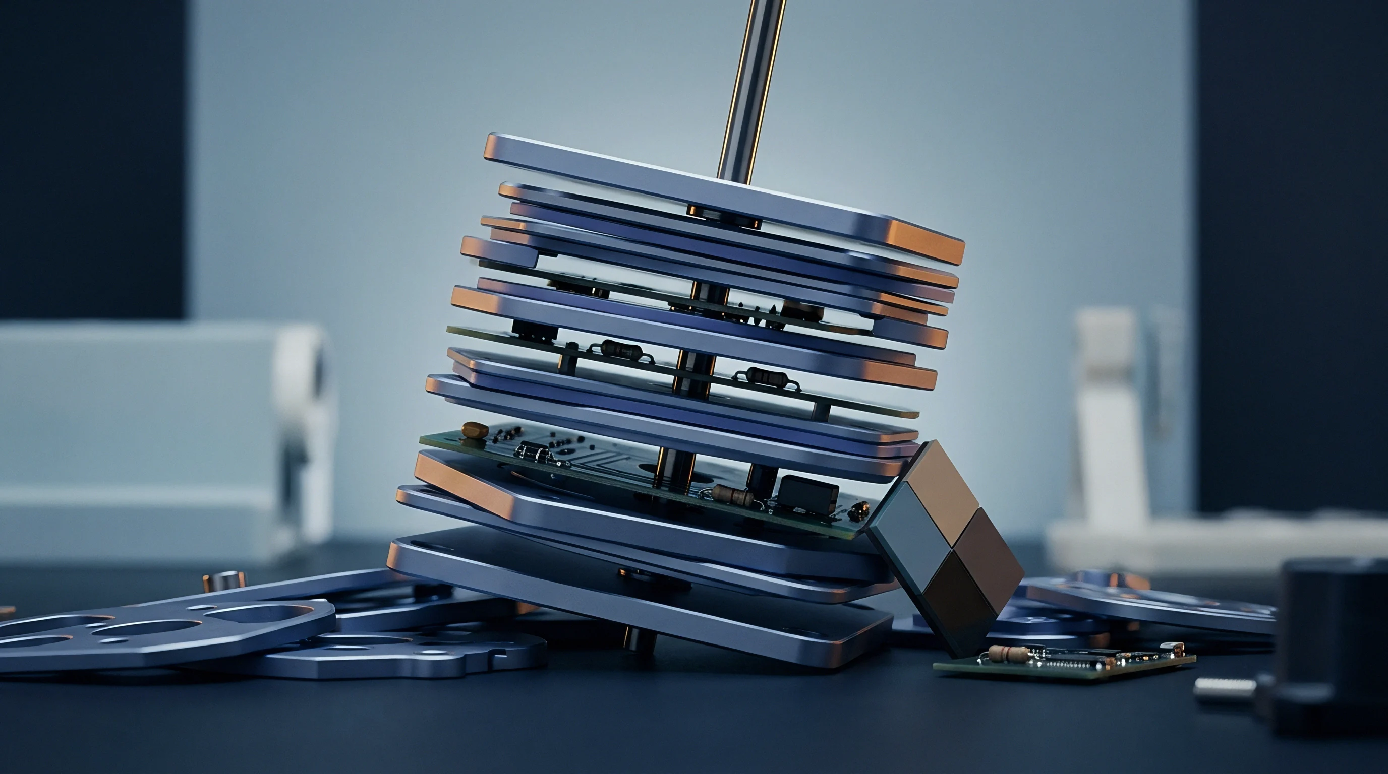
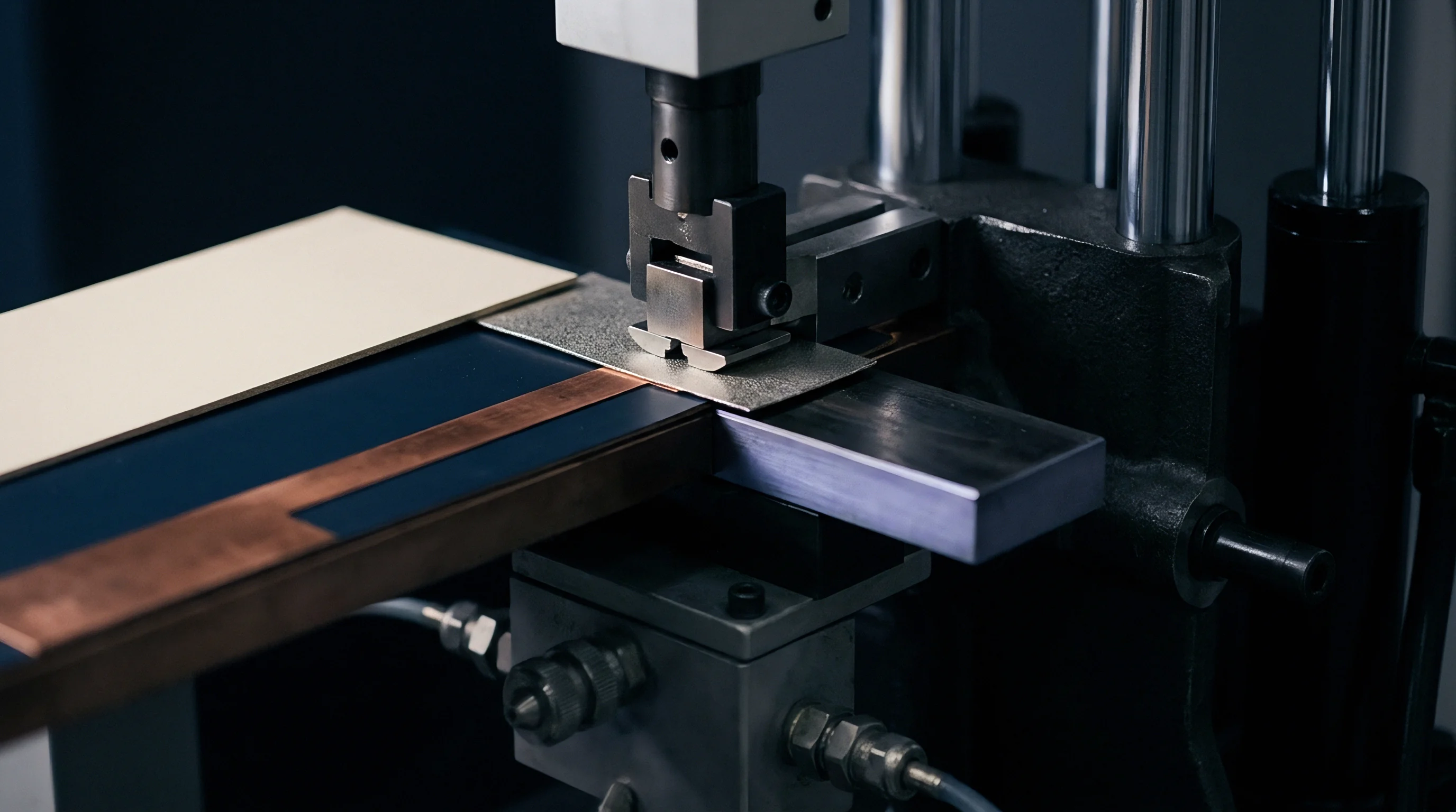
Foil
Electrodeposited copper treatment profiles dictate high-frequency transmission line performance far beyond basic conductivity metrics. Surface topography introduced during foil manufacturing creates microscopic tortuosity that retards signal propagation velocity along stripline trace boundaries. As signal frequency escalates into the gigahertz spectrum, skin depth shrinks below the peak-to-valley roughness dimension of standard electrodeposited copper.
Current flows through the physical contours of the copper treatment rather than a smooth, planar conductor, artificially inflating line resistance and altering the effective dielectric constant experienced by the electromagnetic wave.
Conductor surface roughness directly alters signal phase delay along high-speed traces.
Specification of foil types under IPC-4562 governs both the mechanical tooth depth and the resulting conductor attenuation across high-speed interconnects. Standard electrodeposited copper exhibits a profile height exceeding 6.0 micrometers, which causes severe phase jitter and unmodeled impedance drops in stripline structures operating above 10 GHz. Very Low Profile copper reduces peak roughness below 3.0 micrometers, whereas Hyper Very Low Profile treatment holds surface variation under 1.5 micrometers.
Selecting appropriate foil profiles requires matching microscopic tooth height to the operational wavelength of the signal, preventing unaccounted impedance shifts caused by magnetic field distortion near the conductor surface.
The surface roughness profile of electrodeposited copper alters the internal inductive reactance of a stripline, pulling the phase velocity down and shifting nominal characteristic impedance below theoretical planar calculations.
Chemical bonding treatments applied to core surfaces prior to bonding further complicate the boundary condition. Silane coupling agents and mechanical micro-etching processes increase surface area to ensure peel strength, yet this added micro-roughness degrades high-frequency signal integrity. Electro-deposited treatment steps add lossy metallic oxides or zinc alloy barriers that alter boundary conductivity.
When modeling high-speed striplines, treating the trace as a smooth copper rectangle introduces a systematic error that artificially overstates the actual measured characteristic impedance on a Time Domain Reflectometer.
Chemical etch factors define the final trapezoidal cross-section of the finished conductor.
Etching chemical processes create a trapezoidal trace profile rather than an ideal rectangular cross-section. Spray etchants act longer on the top surface of the copper foil than on the base protected by photoresist, resulting in an inclined sidewall. The ratio of lateral undercut to vertical etch depth defines the etch factor.
Fabricators compensate for this lateral copper loss by increasing nominal artwork trace widths, but variations in etchant chemistry, temperature, and conveyor speed introduce cross-sectional tolerances that directly impact capacitance per unit length.
- Uncalibrated Roughness Models shift effective dielectric constant values upward, driving measured characteristic impedance lower than predicted by planar field solvers.
- Chemical Undercut Variances distort the ratio of top line width to bottom line width, altering localized capacitance along signal paths.
- Oxide Alternative Treatments alter boundary layer conductivity, introducing unpredictable phase velocity shifts across high-frequency differential pairs.
- Asymmetric Foil Selection causes differential warpage during press cycles, introducing mechanical stress that shifts final dielectric thickness distribution.
The interaction between chemical processing and foil selection directly alters impedance tolerance bands. Substrate suppliers offer rolled-annealed, electrodeposited, and reverse-treated foils, each presenting unique tooth structures to the surrounding prepreg. Reverse-treated foil places the smooth drum side of the copper outward while the treated side bonds to the core laminate, modifying the loss characteristics of the lower stripline reference plane.
Ignoring the precise IPC-4562 foil designation within the stackup specification guarantees a mismatch between field solver simulations and coupon measurements.
Foil thickness variations across single panels follow electro-deposition bath current densities. Substrate manufacturers quote nominal copper weights based on mass per unit area rather than absolute physical height. A standard half-ounce copper foil nominally measures 17.5 micrometers in thickness, but processing tolerances under IPC-4562 permit a thickness deviation of up to ten percent.
When combined with localized chemical etching non-uniformities, trace height variability becomes a dominant contributor to impedance tolerance creep in tightly coupled stripline geometries.
Impedance deviations resulting from unverified foil roughness profiles lead directly to expensive fabrication scrap, unaccounted signal reflections, and mandatory board redesigns that ruin project schedules.

Resin
Dielectric substrates specified under IPC-4101 standard slash sheets define the thermal, mechanical, and electrical boundaries of high-speed multilayer printed circuit boards. Glass-reinforced laminates consist of woven fiberglass cloth saturated with thermosetting polymer formulations. The ratio of solid polymer to glass reinforcement directly dictates the relative permittivity and loss tangent of the cured dielectric layer.
Because fiberglass filaments possess a dielectric constant near 5.8 while pure epoxy resin exhibits a value near 3.0, localized resin content variations shift the bulk dielectric constant experienced by stripline traces.
Cured prepreg thickness after lamination rarely matches its initial nominal unpressed height.
Lamination processing transforms fluid prepreg into a cured solid substrate under elevated temperature and vacuum pressure. During this pressing cycle, liquid polymer flows into the interstitial voids between etched copper traces on adjacent inner layers. The volume of copper removed during inner-layer imaging governs the amount of polymer drawn away from the dielectric plane, causing the final pressed prepreg height to drop significantly below its un-pressed nominal thickness.
Stackup designs that fail to account for copper pattern density experience severe dielectric thickness variations, shifting stripline characteristic impedance away from target values.
A material’s dielectric constant changes continuously across the signal frequency spectrum.
Permittivity drops predictably as signal frequency increases due to dipolar relaxation dynamics within the polymer matrix. Material datasheets quoting dielectric constant figures measured strictly at 1 MHz or 1 GHz provide inadequate data for multi-gigabit digital designs. Field solvers must incorporate broadband dielectric models, such as the Svensson-Djordjevic model, which maintain causality by tying frequency-dependent permittivity directly to loss tangent behavior.
Utilizing single-frequency datasheet values for broad-spectrum digital pulses generates substantial mathematical errors in propagation velocity and characteristic impedance calculations.
IPC-4101 slash sheet declarations establish rigid glass-to-resin ratio ranges, where a three percent variation in cured resin content shifts bulk dielectric constant by approximately zero point zero five units.
Glass weave style dictates spatial impedance consistency. Coarse glass fabrics like style 7628 feature thick, tightly twisted yarn bundles separated by wide resin-rich windows. A stripline trace running parallel to the glass yarn matrix experiences a periodic dielectric constant shift as it transitions from traversing solid glass bundles to pure resin gaps.
This spatial variation generates differential phase skew and localized impedance fluctuations. Specifying spread-glass styles such as 1035 or 3313 flattens the yarn profile, creating a uniform dielectric medium that minimizes localized capacitance changes along high-speed signal routes.
| Slash Sheet Standard | Resin Chemistry Type | Glass Transition (Tg) Minimum | Decomposition Temp (Td) Minimum | Dielectric Constant (Dk at 10 GHz) | Dissipation Factor (Df at 10 GHz) |
|---|---|---|---|---|---|
| IPC-4101/24 | Standard Epoxy / Glass | 150 C | 310 C | 4.20 | 0.0200 |
| IPC-4101/99 | Mid-Tg Halogen-Free Epoxy | 150 C | 330 C | 4.00 | 0.0120 |
| IPC-4101/101 | High-Tg Multifunctional Epoxy | 170 C | 340 C | 3.90 | 0.0150 |
| IPC-4101/126 | High-Tg Low-Dk Inorganic Filled | 170 C | 350 C | 3.70 | 0.0090 |
| IPC-4101/131 | High-Speed Low-Loss Polyphenylene Ether | 200 C | 360 C | 3.40 | 0.0040 |
| Data compiled per IPC-TM-650 Method 2.5.5.5 split-post dielectric resonator measurements at 23 degrees Celsius. | |||||
Substrate manufacturers alter inorganic filler loadings to stabilize dielectric properties and control thermal expansion coefficients. Microscopic silica particles dispersed within the matrix reduce overall thermal expansion along the z-axis, preserving plated through-hole integrity during thermal shock. However, non-uniform filler distribution causes localized density gradient fluctuations that introduce micro-scale variations in permittivity.
Evaluating laminate grades under IPC-4101 requires analyzing filler stability under multi-pass reflow conditions to prevent dielectric constant degradation over the operating thermal envelope of the assembly.
Variations in lamination pressure redistribute resin unevenly across the substrate panel.
Substrate flow dynamics during multi-ply lamination demand tight control over press temperature ramp rates and vacuum levels. Excess pressure squeezes polymer out toward panel margins, leaving center zones with higher glass ratios and lower overall dielectric heights. Conversely, insufficient pressure leaves micro-voids around thick inner-layer copper features, degrading dielectric breakdown voltage and creating catastrophic impedance drops.
Fabricators balance prepreg flow behavior against inner-layer copper distribution to maintain consistent z-axis height across every working panel area.
Engineers analyze laminate slash sheets to determine real dielectric boundaries before committing stackup configurations to volume production tooling.
Published dielectric constants represent bare material samples rather than finished laminates, omitting glass pattern variations and fabricator pressing dynamics.
Geometry
Physical dimensions of the stripline cross-section govern electric and magnetic field distribution between upper and lower reference planes. In a symmetrical stripline layout, the signal trace sits centered precisely between two ground planes, bounded by equal dielectric heights above and below. Real-world multilayer fabrication rarely produces perfect symmetry due to operational differences between rigid cured core materials and uncured prepreg plies.
Asymmetrical striplines emerge when prepreg layer thickness differs from core laminate height, introducing complex boundary conditions that require precise numerical modeling.
Reference plane topography directly mirrors underlying copper patterns and copper fills.
Solid ground planes are seldom perfectly flat sheets of metal in dense multilayer designs. Signal traces crossing adjacent power split planes or passing adjacent copper fills encounter step changes in dielectric spacing caused by underlying copper thickness offsets. These physical elevation shifts alter the total distance between the signal trace and its return path, triggering localized characteristic impedance shifts.
Fabricators manage plane flatness by requiring specific copper fill densities on inner layers, preventing reference plane sagging over resin-rich areas.
Does Asymmetrical Cross Section Exacerbate Etch Trajectory Variations?
Trace location within an asymmetrical dielectric cavity alters the electric field density distribution, increasing sensitivity to trace edge profile variations. When a signal conductor approaches one reference plane more closely than the other, capacitance to the nearer plane dominates overall transmission line behavior. Etch factor variations on the trace edge closest to the near reference plane generate larger impedance deviations than equivalent variations in symmetrical configurations.
Fabricators compensate for this heightened sensitivity by narrowing target line width tolerances during chemical imaging steps.
Stripline cross-sectional parameters dictate trace modeling accuracy:
- Bottom Trace Width defines the baseline conductor boundary imaged on the substrate inner layer before chemical etching begins.
- Top Trace Width measures the narrower conductor surface resulting from etchant undercut action during chemical processing.
- Dielectric Cavity Height measures the total distance between upper and lower reference plane copper surfaces after lamination pressure curing.
- Trace Conductive Thickness combines base copper foil height with any additional electro-deposited plating layers added during manufacturing.
- Reference Plane Roughness accounts for the microscopic treatment topography applied to ground plane copper surfaces facing the dielectric cavity.
Dielectric layer compaction during multi-layer press cycles reduces the theoretical distance between inner-layer traces and reference ground planes. Prepreg glass bundles compress against copper trace edges, forcing liquid resin into adjacent channel voids. This physical movement pulls reference planes closer together over dense signal runs while maintaining higher clearance over open field zones.
Field solvers running 2.5D boundary element methods must accept actual microsectioned cross-sectional dimensions rather than idealized artwork specifications to maintain accurate impedance predictions.
Evaluating coupon microsections verifies physical trace geometry against target dimensions calculated during the stackup design phase.
Conductor etch trapezoids alter high-frequency field distribution along signal edges. A lower etch factor produces a sharper top edge, concentrating current flow along tight corner radii due to electrostatic edge effects. This field concentration elevates localized current density, increasing high-frequency conductor loss and slightly pulling characteristic impedance down relative to an ideal rectangular model.
Precision fabrication relies on empirical etch compensation formulas that adjust artwork phototool trace widths to counteract chemical undercut dynamics across varying copper weights.
What structural threshold converts micro-scale cross-sectional dimensional shifts into catastrophic signal phase distortion across ultra-high-speed differential pairs?

Arithmetic
Mathematical modeling of stripline characteristic impedance requires precise analytical closed-form equations or numerical boundary element calculations. Classical stripline formulations derived by Hammerstad and Jensen provide analytical approximations for single stripline geometries based on conductor width, trace thickness, total dielectric spacing, and relative dielectric constant. The basic expression for a symmetrical stripline characteristic impedance (Z0) is represented by:
Z0 = (60 / sqrt(e_r)) ln((1.9 B) / (0.8 W + T))
where e_r represents the bulk relative permittivity, B denotes total dielectric thickness between ground planes, W represents nominal conductor trace width, and T defines total copper trace thickness. Examining this equation reveals that dielectric height B resides in the numerator of the logarithmic argument, making impedance directly proportional to dielectric spacing, while trace width W and thickness T reside in the denominator, rendering impedance inversely proportional to conductor dimensions.
Manufacturing tolerance stackup determines overall printed circuit board production yield.
Calculating the true variance of characteristic impedance requires applying partial differentiation to derive sensitivity factors for each physical parameter. Determining the total differential (dZ0) involves taking the partial derivative of Z0 with respect to each independent variable multiplied by that variable’s individual operational tolerance:
dZ0 = (dZ0 / dW) dW + (dZ0 / dB) dB + (dZ0 / de_r) de_r + (dZ0 / dT) dT
Worst-case analysis assumes that all dimensional variations simultaneously reach their maximum extreme boundaries in directions that combine to maximize overall impedance deviation. While analytically simple, worst-case stackup analysis produces excessively pessimistic tolerance bands that force unrealistically tight fabrication limits, escalating bare board costs unnecessarily.
Root-Sum-Square statistical modeling assumes that individual manufacturing process variations follow independent normal distributions. Root-Sum-Square calculations combine parameter variances using the square root of the sum of squared partial derivative product terms:
sigma_Z0 = sqrt( ((dZ0 / dW) sigma_W)^2 + ((dZ0 / dB) sigma_B)^2 + ((dZ0 / de_r) sigma_e_r)^2 + ((dZ0 / dT) sigma_T)^2 )
Evaluating this statistical model reveals that dielectric thickness variation (σB) and line width variation (σW) dominate the total impedance variance, whereas copper thickness variation (σT) contributes a smaller percentage to overall deviation in standard stripline structures.
| Physical Parameter | Nominal Design Value | Manufacturing Tolerance Range | Partial Derivative Sensitivity (dZ0 / dX) | Percentage Contribution to Total Z0 Variance |
|---|---|---|---|---|
| Dielectric Height (B) | 0.250 mm | +/- 0.0125 mm | +142.5 ohm/mm | 52.4% |
| Trace Width (W) | 0.125 mm | +/- 0.0075 mm | -185.0 ohm/mm | 31.2% |
| Relative Permittivity (e_r) | 3.80 | +/- 0.150 units | -6.58 ohm/unit | 11.8% |
| Copper Thickness (T) | 0.0175 mm | +/- 0.0020 mm | -112.0 ohm/mm | 4.6% |
Calculating root sum square variations across production batches establishes realistic engineering tolerance limits before releasing final manufacturing drawings.
Consider a practical engineering scenario involving a target 50-ohm single-ended stripline designed on a high-speed low-loss material system. The nominal stackup parameter targets are set as follows: total dielectric height B equals 0.250 mm, nominal line width W equals 0.125 mm, copper thickness T equals 0.0175 mm (1/2 oz foil), and relative permittivity e_r equals 3.80 at 10 GHz. Plugging these base parameters into the analytical model yields a baseline characteristic impedance (Z0) of precisely 50.12 ohms.
Pessimistic worst-case models artificially drive up board manufacturing costs.
Applying standard PCB fabrication tolerances under IPC-6012 Class 2 execution modifies these inputs across defined production bounds. Dielectric height B varies by five percent (+/- 0.0125 mm), line width W varies by +/- 0.0075 mm due to etch undercut non-uniformity, relative permittivity e_r varies by +/- 0.15 units across resin lots, and copper thickness T varies by +/- 0.0020 mm. Calculating extreme worst-case upper bound condition forces B to 0.2625 mm, W to 0.1175 mm, e_r to 3.65, and T to 0.0155 mm, which elevates the maximum calculated impedance to 56.45 ohms.
Conversely, forcing lower bound parameters drops calculated impedance to 44.18 ohms. This worst-case analysis indicates a total impedance spread of +/- 6.135 ohms (+/- 12.24 percent), exceeding standard ten percent specification windows.
A nominal 50-ohm stripline stackup subject to three-sigma manufacturing variations under IPC-6012 Class 2 yield limits exhibits a statistical Root-Sum-Square impedance spread of plus or minus 3.12 ohms.
Applying Root-Sum-Square statistical combinations to the same manufacturing tolerance inputs provides a much more accurate representation of volume production yields. Evaluating partial derivatives at nominal conditions yields: dZ0/dB equals +142.5 ohms/mm, dZ0/dW equals -185.0 ohms/mm, dZ0/de_r equals -6.58 ohms/unit, and dZ0/dT equals -112.0 ohms/mm. Multiplying these sensitivity coefficients by their respective three-sigma process standard deviations and taking the square root of the sum of squares yields a statistical three-sigma impedance deviation of +/- 3.12 ohms (+/- 6.22 percent).
This demonstrates that statistical process control yields acceptable production rates within a standard +/- 10 percent target specification without forcing overly restrictive drawing requirements.
Executing an analytical stackup tolerance evaluation requires a systematic mathematical workflow:
- Establish baseline target characteristic impedance using a validated field solver or analytical stripline equation with nominal material dimensions.
- Extract exact manufacturing tolerance ranges for copper thickness, etch undercut, prepreg pressed height, and relative permittivity from the target fabricator process capability data.
- Compute numerical partial derivatives for characteristic impedance with respect to each independent physical variable at the nominal operating point.
- Calculate individual variance product terms by multiplying each partial derivative by its associated process standard deviation.
- Sum the squared variance terms and calculate the square root to determine the total expected statistical impedance standard deviation.
- Compare three-sigma statistical impedance limits against customer design specifications to verify expected panel yield rates.
Differential stripline configurations introduce mutual edge coupling parameters that expand the analytical matrix. Differential impedance (Zdiff) depends on single-ended characteristic impedance (Z0) and edge-to-edge trace spacing (S). The mathematical relationship is expressed by:
Z_diff = 2 Z0 (1 – 0.374 exp(-2.9 S / B))
Variation in trace spacing S directly influences the coupling coefficient. As trace spacing shrinks to achieve tighter spatial routing density, sensitivity to trace spacing tolerances (dS) escalates dramatically, making trace registration and imaging accuracy the primary drivers of differential impedance drift.
Per IPC-6012 Clause 3.6.2.8, characteristic impedance tolerance compliance must be verified using dedicated test coupons located on panel margins, where measured values must fall within the specified percentage window of nominal drawing targets.

Bench
Physical verification of stripline impedance requires empirical testing of standardized coupon structures using specialized high-frequency instrumentation. Time Domain Reflectometry operates by launching a fast electrical step function down a test transmission line and measuring reflected voltage amplitudes over time. Discontinuities in characteristic impedance produce reflected voltage steps proportional to the reflection coefficient (Γ).
The measured reflection coefficient maps directly to local impedance values along the length of the signal path, revealing exact spatial locations where dimensional variations occur.
Test coupons must reflect the exact physical environment of functional board circuitry.
Test coupons positioned on outer panel margins experience slightly different etching and lamination conditions than signal paths located near panel centers. Fluid dynamics during chemical spraying cause etchant pooling near panel edges, creating edge-to-center trace width variations. Furthermore, lamination press pressure distributions often drop near outer margins, leading to thicker dielectric layers on test coupons relative to functional active circuitry.
Accurate bench correlation mandates placing test coupons within working board areas or applying empirical offset factors that account for margin process variances.

What Launch Artifacts Corrupt Time Domain Reflectometry Microsection Data?
Probe launch discontinuities introduce high-frequency parasitic inductance and capacitance that mask true stripline impedance profiles near the start of a signal route. Pogo-pin test fixtures and coaxial SMA launches create localized impedance spikes caused by unshielded center conductor lengths and ground-loop inductance. Time Domain Reflectometry algorithms apply time-gating windows to isolate launch artifacts, but setting the measurement gate too close to the connector boundary yields false impedance readings distorted by settling transients.
Empirical impedance verification relies on established standard test methods and documentation frameworks:
- IPC-TM-650 Method 2.5.5.7 defines single-ended and differential characteristic impedance measurement procedures using Time Domain Reflectometry instruments.
- IPC-TM-650 Method 2.5.5.12 details split-post dielectric resonator procedures for extracting real relative permittivity and dissipation factor values from cured laminates.
- Microsection Verification Inspection Reports document physical trace top width, bottom width, copper thickness, and dielectric spacing captured via optical metrology.
- Coupon Trace Artwork Cross-References record exact layout dimensions, reference plane clearances, and panel locations for every measured test line.
Unmodeled dielectric compression adjacent to inner-layer ground fills produces an offset of up to 3.8 ohms during lamination validation.
Cross-section microsectioning serves as the ultimate physical audit for validating theoretical stackup models against cured circuit boards. Optical microscopes measure trace edge angles, core dielectric heights, prepreg fill profiles, and copper foil treatment structures at multi-hundred-times magnification. Comparing microsection measurements directly against Time Domain Reflectometry impedance traces highlights specific process variations, such as localized resin starvation or reference plane tilt, enabling rapid recalibration of field solver stackup parameters.
Single-ended Time Domain Reflectometry traces measured without adjusting for launch probe inductance yield artificially elevated impedance spikes during the first one hundred picoseconds of signal propagation.
Uncalibrated field solvers produce flawed simulations that lead directly to scrap production runs.
Field solver software tools rely on user-entered physical inputs to generate mathematical transmission line models. When designers enter nominal datasheet dielectric constant values and ideal rectangular trace geometries into simplified 2D field solvers, predicted impedance results diverge from physical bench measurements. Advanced 2.5D and 3D electromagnetic field solvers incorporate real microsection profiles, frequency-dependent dielectric loss models, and surface roughness variables to align theoretical predictions with actual bench test results.
Bench measurement accuracy relies on maintaining probe contact pressure consistent with calibrated calibration substrate standards.
Ledger
Specification decisions fixed on the assembly drawing dictate manufacturing yield rates, factory selection options, and ultimate unit pricing for bare circuit boards. Ordering stripline stackups with unnecessarily restrictive impedance tolerances drives fabrication scrap up, forcing vendors to build risk premium margins directly into their base quotations. Standard commercial fabrication achieves +/- 10 percent impedance tolerances comfortably under basic statistical process controls, whereas tightening tolerances to +/- 5 percent limits the qualified vendor pool and triggers significant pricing multipliers.
Panel area utilization and manufacturing yield directly dictate per-unit board prices.
Bare board production costs depend fundamentally on panel area utilization efficiency. Fabricators process standard production panel sizes, such as 18 by 24 inches, squeezing as many individual board arrays onto a single panel as mechanical clearances permit. Imposing ultra-tight impedance tolerances forces fabricators to enlarge outer margin test coupon zones and expand spacing between adjacent boards to balance thermal flow during lamination, reducing total array density per panel and elevating cost per delivered unit.
| Fabrication Specification Level | Impedance Tolerance Capability | Dielectric Height Control Range | Etch Width Tolerance Limit | Relative Unit Cost Multiplier | Estimated Production Panel Yield |
|---|---|---|---|---|---|
| IPC-6012 Class 2 Standard | +/- 10% Nominal | +/- 10% Nominal Height | +/- 0.0125 mm | 1.00x Base Price | 98.5% Yield |
| IPC-6012 Class 3 High Reliability | +/- 8% Nominal | +/- 7% Nominal Height | +/- 0.0085 mm | 1.35x Base Price | 94.0% Yield |
| Precision High-Speed Spec | +/- 5% Nominal | +/- 4% Nominal Height | +/- 0.0050 mm | 2.10x Base Price | 82.0% Yield |
| Ultra-Tight Advanced Spec | +/- 3% Nominal | +/- 2% Nominal Height | +/- 0.0025 mm | 4.50x Base Price | 58.0% Yield |
Strict impedance targets frequently force a switch to high-cost substrate materials.
Achieving impedance tolerances tighter than +/- 5 percent forces switchover from standard FR-4 materials specified under IPC-4101/24 to specialized low-loss PTFE or hydrocarbon material systems specified under IPC-4101/131. Premium raw laminates carry raw material cost multipliers ranging from three to eight times baseline epoxy prices. Furthermore, these advanced resin matrices require specialized chemical processing steps, extended lamination bake cycles, and specialized diamond-coated cutting tools, compounding total manufacturing costs across every production batch.
Procurement specifications that designate exact slash sheet numbers without defining allowable material substitution bands create expensive supply chain bottlenecks. Standardizing on common, widely stocked slash sheets like IPC-4101/126 or IPC-4101/131 allows fabricators to source materials from multiple qualified laminate vendors without requiring formal engineering drawing revisions. Open laminate cross-reference lists preserve purchasing flexibility while holding physical dielectric properties strictly within calculated engineering limits.
Yield loss calculations must include the compound effect of multi-layer registration errors on complex high-layer-count stripline boards. As layer counts increase beyond sixteen layers, thermal expansion mismatch during sequential lamination cycles degrades inner-layer feature alignment. Misregistered signal traces moving relative to underlying reference plane splits trigger catastrophic localized impedance drops that result in panel rejection during final automated optical inspection and TDR testing.
Balancing financial risk against electrical performance demands that design engineers reserve tight +/- 5 percent impedance tolerances exclusively for critical high-speed differential pairs while maintaining standard +/- 10 percent windows across general parallel bus topologies. Fabricators welcome hybrid tolerance specifications on fabrication drawings, provided clear net class definitions identify which specific signal paths mandate precision processing. Aligning drawing notes directly with factory process capabilities maximizes panel yield, lowers bare board procurement unit costs, and guarantees consistent signal integrity across high-volume production runs.