Evaluating in Plane Permittivity Impact on Differential Fringing Fields
Evaluating in-plane permittivity accounts for horizontal field concentration in edge-coupled pairs, preventing 2 to 5 ohm impedance drops in high-density boards.

Weave
Dielectric Anisotropy in Glass Reinforced Substrates
Woven fiberglass laminates show directional differences in relative permittivity because continuous E-glass or L-glass fibers run along set axes within an epoxy, cyanate ester, or polyphenylene ether resin matrix. Continuous glass filaments have an isotropic relative permittivity of 6.1 to 6.6, while cured thermosetting resin systems sit lower, between 2.8 and 3.2 at 10 GHz. Weaving dense fiber bundles in warp and fill directions turns the composite dielectric into an anisotropic tensor.
Out-of-plane permittivity ~ the vertical component perpendicular to the laminate surface ~ sees a lower effective glass fill factor because field lines cross alternating resin-rich and glass-rich layers, with the glass filaments directing the electric flux.
In-plane permittivity covers the orthogonal directions parallel to the board surface, where electric fields follow uninterrupted continuous glass strands. Fields oriented parallel to the laminate reinforcement encounter a parallel-capacitance physical arrangement, whereas fields normal to the board surface see a series stackup. Because of that structural difference, in-plane relative permittivity exceeds out-of-plane relative permittivity by 10 percent to 22 percent, depending on glass style, yarn bundle flattening, and resin content percentage.
Standard IPC-4101 slash sheets report dielectric constants extracted strictly through out-of-plane test geometries. Designers and fabricators who plug those single-axis numbers into two-dimensional field solvers assume isotropic material behaviour. That assumption breaks down on dense differential pairs with sub-100 micrometre trace separation, where horizontal electric field coupling governs line behavior and introduces impedance deviations from target specifications.
Glass Style Influence on Planar Vectoring
Fiber bundle selection governs the physical spacing between glass strands and internal resin pockets. Heavy square weaves such as 7628 use thick yarn bundles that leave pronounced resin-rich windows between warp and fill intersections. Finer fabrics including 1035, 1067, and 1078 feature flattened bundles that close those voids, distributing glass far more uniformly across the plane of the sheet.
Spread-glass styles decrease local dielectric variations beneath signal traces, but they maximize the total horizontal glass volume fraction relative to resin pockets. High glass density parallel to the trace surface elevates in-plane permittivity above values measured on looser, open glass structures.
| Glass Style | Resin Content Percentage | Out Of Plane Permittivity | In Plane Permittivity | Anisotropy Factor Ratio |
|---|---|---|---|---|
| 1035 Spread Glass | 72% | 3.25 | 3.58 | 1.101 |
| 1078 Spread Glass | 64% | 3.38 | 3.82 | 1.130 |
| 2116 Standard Weave | 54% | 3.65 | 4.23 | 1.158 |
| 7628 Standard Weave | 42% | 4.10 | 4.92 | 1.200 |
Laminate suppliers adjust resin formulations primarily to control z-axis thermal expansion during solder reflow cycles. Raising resin content lowers out-of-plane permittivity because thermoset polymers have lower dielectric constants than silica glass, but it also alters the ratio between horizontal and vertical field velocities across high-frequency transmission channels.
Planar dielectric divergence develops during prepreg treater processing and multi-platen hydraulic press consolidation:
- Glass filament alignment occurs under mechanical tension during raw fiber yarn preparation, establishing continuous high-permittivity conductive paths along the horizontal axes.
- Hydrostatic resin displacement forces low-dielectric polymer matrices into interlaminar spaces during hot press cycles, creating distinct resin-rich layers between woven reinforcement sheets.
- Silane coupling agent chemistry creates a microscopic boundary layer between glass filaments and resin, altering localized dielectric polarization mechanisms along the fiber surface.
- Thermal shrinkage differential induces micro-scale stress patterns during cooling, subtly altering local material density along horizontal fiber paths.
When predicted differential impedance misses laboratory TDR measurements, material vendors often attribute the discrepancy to trapezoidal copper foil profiling or prepreg pressing tolerances rather than reporting anisotropic permittivity parameters on master material specification sheets.
Fringe
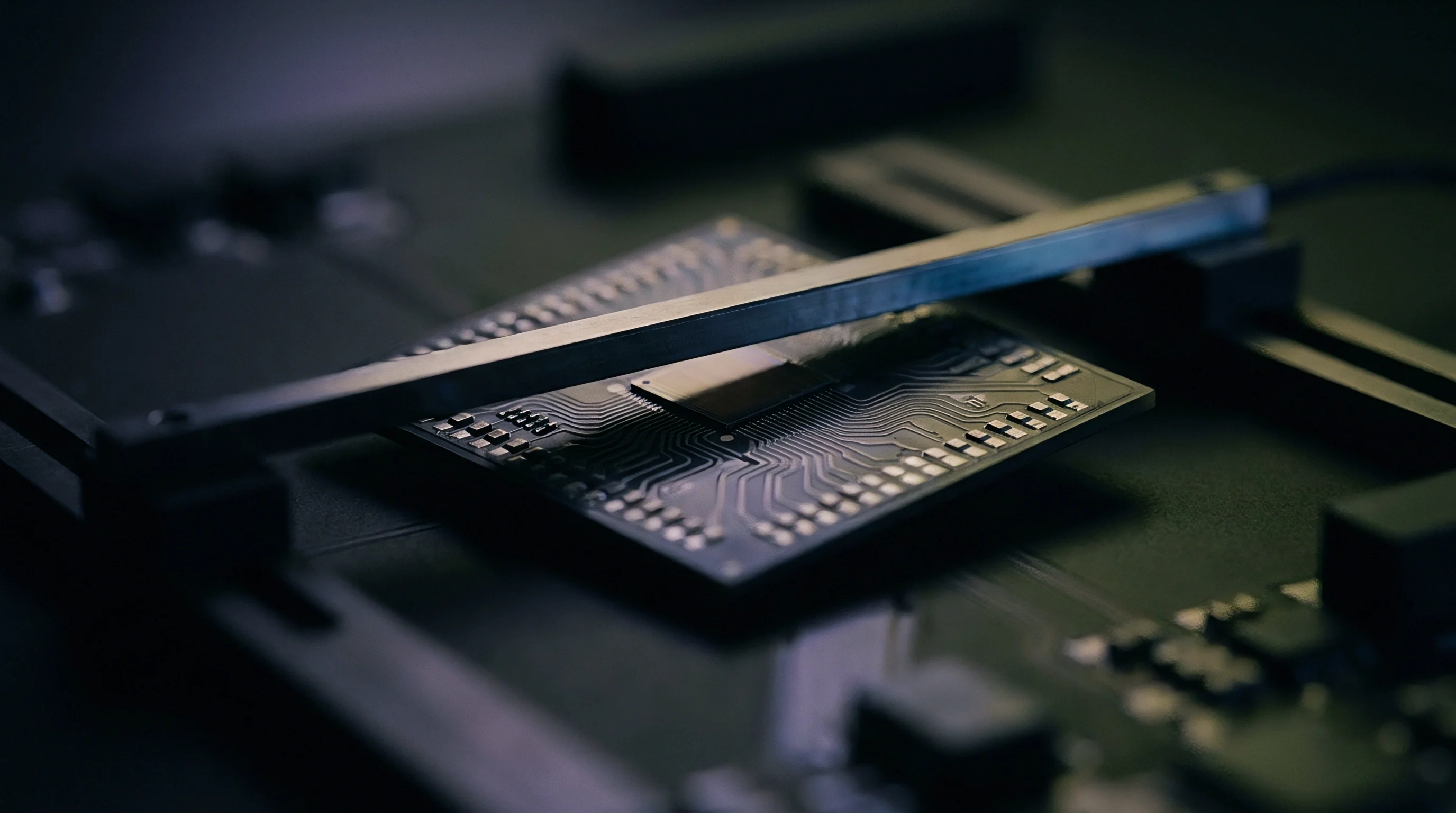
Odd Mode Electric Field Distribution in Edge Coupled Pairs
Differential signaling relies on two tightly coupled conductors carrying equal-amplitude signals with opposite phase polarity, where total differential impedance equals twice the odd-mode impedance of a single conductor. Odd-mode excitation sets up a virtual ground plane midway between the two conductors. This zero-potential boundary pulls electric field lines horizontally outward from the inner sidewall of each trace toward the opposing conductor.
On tightly coupled differential microstrip and coplanar structures where edge-to-edge separation drops below trace width, odd-mode fringing fields concentrate heavily within the horizontal dielectric volume between trace edges. While single-ended microstrips send electric fields vertically down to the ground plane through the out-of-plane dielectric, differential fringing lines cut across the top horizontal substrate layer before curving downward.
Equally spaced differential traces running over anisotropic glass reinforcement display odd mode velocity shifts proportional to trace sidewall proximity.
When horizontal electric flux passes through a material whose in-plane permittivity exceeds its out-of-plane permittivity, total odd-mode capacitance per unit length increases beyond isotropic model estimates. That additional capacitance depresses both odd-mode impedance and differential impedance below calculated target figures.
Capacitance Tensor Effects on Coplanar Waveguides
Grounded coplanar waveguide structures with narrow air gaps show extreme sensitivity to in-plane permittivity values. Placing coplanar reference ground traces directly alongside signal lines forces electric flux laterally across the horizontal substrate interface. Because the air above provides a fixed dielectric constant of 1.0, the internal horizontal substrate path becomes the dominant determinant of line capacitance.
Anisotropic permittivity splits signal velocity components between odd and even propagation modes. Even-mode excitation drives electric fields vertically toward the underlying ground reference plane, interacting primarily with out-of-plane permittivity, whereas odd-mode excitation directs fringing flux horizontally through the higher in-plane dielectric.
Phase velocity equals the speed of light divided by the square root of effective permittivity. Because odd and even modes interact with different dielectric tensor components, their effective dielectric constants diverge. That mismatch generates mode conversion, transforming differential signal energy into common-mode noise that cuts into receiver eye margins and risks failing electromagnetic interference compliance limits.
Routing high-speed serial links with tight differential spacing on laminates with uncharacterized in-plane dielectric constants risks systematic impedance undershoot ~ routinely yielding 85 ohm differential channels on layouts designed for 90 ohms, which triggers reflection penalties at high data rates.
Benchmark

In Plane Dielectric Measurement Standard Methods
Characterizing in-plane permittivity requires test fixtures that direct electric field vectors purely parallel to laminate surfaces. Standard out-of-plane techniques, such as IPC-TM-650 Method 2.5.5.5 using a split-post dielectric resonator or Method 2.5.5.13 using a clamped stripline fixture, orient electric fields normal to the sample face. These out-of-plane configurations leave horizontal tensor properties completely obscured.
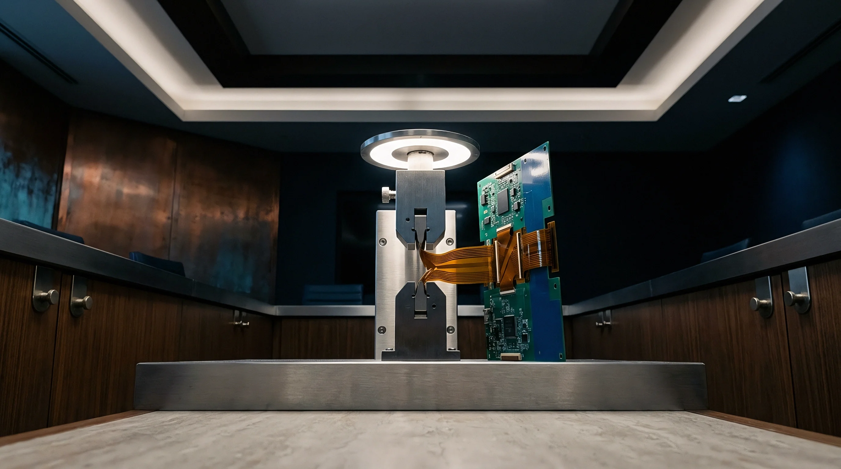
IPC-TM-650 Method 2.5.5.12 specifies an in-plane stripline resonator evaluation procedure. The test sample is machined into narrow dielectric strips stacked vertically inside a resonant cavity, which aligns the original planar laminate axes parallel to the cavity’s electric field excitation vector. Resonance frequency shifts then allow extraction of in-plane permittivity across frequencies from 1 GHz to 10 GHz.
Bereskin stripline fixtures and split-cavity resonators offer alternative extraction pathways. These fixtures utilize thin, unclad laminate coupons, measuring quality factor and phase shift changes within high-frequency TE-mode resonant cavities. Accurate extraction requires precise sample thickness measurement, as micrometer errors artificially skew calculated in-plane dielectric numbers.
Does in Plane Testing Expose Batch Dielectric Variance?
Raw material manufacturers perform lot-acceptance dielectric testing using automated split-post resonators for speed and minimal sample preparation. Split-post testing isolates vertical dielectric properties, but it misses horizontal material fluctuations caused by glass yarn tension variations during weaving.
In-plane testing exposes substrate batch variations that vertical testing masks. Changes in silane size chemistry, yarn flattening pressure, or prepreg resin flow modify horizontal dielectric performance while leaving vertical test metrics within published specification limits. Stackup engineers verifying low-loss substrates inspect both orthogonal dielectric values to validate signal line models prior to high-volume fabrication release.
- Out-of-plane SPDR testing measures vertical dielectric constants at fixed frequencies quickly without destructive sample preparation, serving standard slash sheet baseline generation.
- In-plane stripline resonator testing measures horizontal dielectric tensor components accurately by rotating material sample geometry inside resonant microwave cavities.
- Full-wave 3D TDR extraction back-calculates anisotropic material properties from fabricated coupon propagation delay measurements across multiple line spaces.
- Split-cavity perturbation fixtures evaluate unclad thin core substrates across wide thermal cycles to map temperature-dependent planar dielectric drift.
Master purchase agreements specifying high-frequency laminates reference IPC-4101 parameters, but incorporating explicit line items requiring periodic IPC-TM-650 2.5.5.12 in-plane test reports forces raw material mills to hold horizontal dielectric tolerance bands within plus or minus 0.05 of nominal design targets.
Calculation
Field Solver Discrepancy in Edge Coupled Pairs
Evaluating the mathematical impact of in-plane permittivity requires comparing a standard isotropic two-dimensional field solver prediction against a three-dimensional anisotropic field solver model. Take an edge-coupled microstrip differential pair routed on the outer layer of a high-speed circuit board over an internal ground reference plane.
Assume a target differential impedance of 90.0 ohms. Set trace width at 125 micrometres, trace copper thickness at 30 micrometres with half-ounce electrodeposited foil, trace sidewall profile trapezoidal with a 60-degree edge taper, dielectric height above reference plane at 100 micrometres, and trace edge-to-edge separation at 100 micrometres. The core material is a spread-glass low-loss laminate with an out-of-plane permittivity of 3.40 measured at 10 GHz via split-post dielectric resonator.
An isotropic 2D solver uses 3.40 for all field directions. It calculates single-ended impedance at 56.2 ohms, odd-mode impedance at 45.0 ohms, and differential impedance at 90.0 ohms. Line capacitance per unit length breaks down into vertical capacitance to ground and horizontal mutual capacitance between traces.
An anisotropic 3D solver incorporates the true material properties: out-of-plane permittivity remains 3.40, but in-plane permittivity measures 3.85 based on IPC-TM-650 2.5.5.12 testing due to continuous glass filament alignment. The anisotropic solver recalculates line parameters under tensor equations.
| Parameter Description | Isotropic Model (E_z = 3.40, E_xy = 3.40) | Anisotropic Model (E_z = 3.40, E_xy = 3.85) | Absolute Variance | Percentage Delta |
|---|---|---|---|---|
| Single Ended Impedance | 56.2 Ohms | 55.1 Ohms | -1.1 Ohms | -1.96% |
| Odd Mode Impedance | 45.0 Ohms | 42.8 Ohms | -2.2 Ohms | -4.89% |
| Even Mode Impedance | 68.1 Ohms | 67.4 Ohms | -0.7 Ohms | -1.03% |
| Differential Impedance | 90.0 Ohms | 85.6 Ohms | -4.4 Ohms | -4.89% |
| Odd Mode Velocity | 1.72 x 10^8 m/s | 1.64 x 10^8 m/s | -0.08 x 10^8 m/s | -4.65% |
Horizontal dielectric permittivity increases mutual fringing capacitance between the conductors by 12.8 percent. Higher mutual capacitance depresses odd-mode impedance from 45.0 ohms down to 42.8 ohms. Differential impedance drops from the 90.0 ohm target down to 85.6 ohms, introducing a 4.4 ohm error that exceeds standard 5 percent board fabrication tolerances before manufacturing geometric variations occur.
Anisotropic dielectric modeling shifts calculated differential impedance by 4.4 ohms on tight 100 micrometre edge-coupled lines at 10 GHz.
Etching processes produce trapezoidal trace cross-sections where bottom copper widths exceed top copper widths. These trapezoidal profiles narrow the top edge-to-edge separation gap between adjacent conductors, concentrating horizontal electric field lines near the upper corners of the copper traces and amplifying in-plane permittivity sensitivity.
Mode Conversion Induced by Dielectric Asymmetry
Differential transmission lines require symmetrical phase velocities to prevent mode conversion. When signal traces run at an angle relative to the underlying glass fabric weave, one conductor sits over a resin-rich weave intersection while the sibling conductor sits directly over a dense glass yarn bundle.
This positional asymmetry combines with in-plane dielectric anisotropy to alter the local odd-mode effective dielectric constant independently for each line in the pair. The skew converts differential energy into common-mode noise according to mixed-mode S-parameter conversion calculations:
SCD21 = 0.5 (S21 – S11 + S22 – S12) sin(delta_phi)
Here delta_phi represents the phase delay difference accumulated between the two signal lines over line propagation distance. Higher in-plane permittivity accelerates phase delay divergence along the line, causing S-parameter mode conversion losses to cross compliance threshold limits over shorter interconnect lengths.
This mathematical divergence leaves an open question regarding how stackup modeling software can dynamically ingest localized microsectioning data from pressed production panels to continuously update 3D field solver tensor inputs across varying production lots.
Drawing
Stackup Specification Rules for Anisotropic Laminates
Fabrication drawings serving high-density board orders require precise material control notes to prevent unapproved laminate substitutions. Standard stackup drawings specify dielectric thickness, nominal copper weight, and target single-ended or differential impedance numbers, leaving laminate selection to fabricator engineering teams.
Engineering release packages targeting high-frequency, tightly coupled differential architectures specify both material slash sheet designations and explicit anisotropic permittivity bounds within stackup notes. Specifying out-of-plane permittivity without constraining in-plane permittivity permits fabricators to substitute glass weave styles to adjust press-thickness targets, altering differential line coupling without violating drawing thickness parameters.
Fabrication master notes specify laminate slash sheet, glass style weave count, and target impedance coupons simultaneously.
Impedance coupon designs placed on production panel borders reflect the exact geometric cross-sections released in board artwork files. Standard impedance coupons measure single-ended striplines or widely spaced differential lines, failing to detect in-plane dielectric coupling variations that manifest on dense internal signal layers.
Production File Documentation Protocol
Releasing production artwork and stackup drawings to bare-board suppliers follows an established documentation flow to lock down physical material properties:
- Define nominal dielectric thickness, foil copper weight, and glass weave style for every prepreg and core layer on the stackup drawing sheet.
- Mandate anisotropic material modeling using both vertical and horizontal permittivity input fields inside full-wave 3D field solver software during preliminary design rule generation.
- Add explicit fab drawing notes restricting laminate substitution to pre-qualified slash sheets with published in-plane dielectric properties matching IPC-TM-650 2.5.5.12 test data.
- Design dedicated differential impedance test coupons incorporating maximum edge-coupling trace densities matching critical internal layer signal geometries.
- Require fabricators to supply TDR microsection verification reports confirming final etched trace cross-section geometry, top and bottom trace widths, and dielectric height after multi-platen pressing.
While coupons verify etched trace profiles, panel layout drawings that specify edge-coupled impedance targets require fabricator engineering queries to clear field solver discrepancies before cutting raw core stock.
A simple operational guideline governs high-density differential stackup release: tighten trace spacing only after confirming the fabricator field solver incorporates in-plane dielectric parameters.
Discrepancy

Commercial Yield and Landed Cost Analysis
Accounting for in-plane permittivity within high-density differential designs influences total landed PCB cost by governing scrap rates, raw material selection, and panel utilization metrics. Standard FR-4 materials sell near $15 to $22 per working panel, whereas mid-loss materials like Megtron 4 range from $38 to $55 per panel. Ultra-low-loss materials including Megtron 6, Tachyon 100G, or Rogers 4000 series cost between $85 and $180 per panel.
Designing tight differential channels using isotropic field solvers creates an immediate yield risk during final coupon testing. When a fabricator builds panels to an uncompensated artwork geometry, TDR coupon measurements reveal differential impedance sitting 4 to 5 ohms below target limits. The factory attempts to restore impedance by over-etching copper traces to reduce line width, reducing signal conductor cross-sections.
Over-etching trace widths to raise line impedance reduces circuit yield. Etching a 100 micrometre trace down to 88 micrometres increases line resistance, introduces trace width variance along the line length, and breaches IPC-6012 Class 3 minimum conductor width requirements. Reduced trace width yield losses push batch scrap rates from a baseline 2 percent up to 14 percent, inflating unit board costs across production runs.
| Material Grade | Material Panel Cost | Modeling Strategy | Etch Adjustment Risk | Panel Yield Rate | Landed Board Unit Cost |
|---|---|---|---|---|---|
| Standard High-Tg FR-4 | $24.50 | Isotropic 2D Solver | Severe Over-Etching Required | 81.5% | $18.40 |
| Mid-Loss Spread Glass | $48.00 | Isotropic 2D Solver | Moderate Over-Etching Required | 88.2% | $21.15 |
| Mid-Loss Spread Glass | $48.00 | Anisotropic 3D Solver | Zero Geometry Adjustment | 97.4% | $19.20 |
| Ultra-Low-Loss PTFE Base | $142.00 | Anisotropic 3D Solver | Zero Geometry Adjustment | 98.1% | $38.60 |
While yield often drops on thin cores, upgrading from standard glass fabrics to low-anisotropy spread-glass laminates increases raw material cost per panel by $20 to $30. Accurate anisotropic dielectric modeling on mid-loss spread-glass substrates delivers higher total panel yield, offsetting initial material cost premiums by eliminating scrap penalties.
Panel Utilization Mechanics and Factory Queries
Adjusting edge-coupled trace separation during artwork compensation alters trace-to-trace clearance rules across dense BGA breakout regions. Widening trace separation by 15 micrometres to counter in-plane permittivity capacitance drops forces layout engineers to add signal layers to maintain routing density. Moving a design from a 12-layer stackup to a 14-layer stackup increases panel press cycles and raises base panel price by 18 percent to 24 percent.
When fabricators receive manufacturing files generated with isotropic field solver models, engineering queries delay job release into production. The fabricator’s CAM department identifies the 4 ohm predicted undershoot on tight differential pairs and issues a formal engineering query requesting artwork modifications, trace widening, or dielectric layer substitution.
Resolving engineering queries takes two to five business days, consuming fast-turn quick-turn schedule buffers and risking assembly line downtime. Correcting field solver algorithms prior to Gerber release prevents engineering queries, stabilizes factory tooling pipelines, and secures target panel delivery schedules.
Selecting spread glass laminates with characterized in-plane permittivity vectors stabilizes differential coupling, holds TDR coupon measurements inside tight 5 percent tolerance windows, and optimizes delivered working boards per panel across volume manufacturing runs.