Measuring Dielectric Constant Variance across Woven Glass Laminate Panels
Spatial resin flow and glass weave density variations across woven laminate panels drive localized dielectric drift, requiring strict test protocols and explicit stackup drawing bounds.

Resin
Long before a high-frequency signal reaches a trace, a bare laminate panel on an assembly line already has shifting dielectric constants across its surface. Continuous glass filaments with a relative permittivity near 6.6 sit embedded in an epoxy polymer matrix closer to 3.0. The cured composite’s overall relative permittivity depends on the local ratio between these two phases.
As prepreg flows under heat and clamping force in a multi-platen press, fluid polymer shifts relative to the rigid woven glass. A three percent matrix density gradient across an eighteen by twenty-four inch sheet can shift localized phase velocity enough to push controlled-impedance lines past commercial limits.
The nominal value on a datasheet is just a macro-scale average from lab measurements. Manufacturing these laminates means combining glass yarns woven at right angles with semi-cured liquid polymer. Bundle density, filament count, and treater tension set the starting ratio of glass to resin binder.
Structural variations start during core pressing, when pressure gradients force resin outward toward the sheet’s outer edges. The center of a large production sheet holds a slightly higher polymer-to-glass ratio than the perimeter, driving a systematic radial shift in effective permittivity.
Local variations in permittivity develop through several physical mechanisms during fabrication and pressing:
- Glass Thread Count Variation shifts spatial density where warp and weft bundles cross, altering local phase velocity along parallel routing channels.
- Hydrophobic Matrix Aging causes uneven moisture absorption during air exposure, raising dielectric values locally because of water’s high permittivity.
- Hydrostatic Pressure Gradients across pressing platens push liquid prepreg into low-density zones, changing pressed thickness and the local resin-to-glass ratio across the panel.
- Chemical Cross-Linking Heterogeneity during thermal curing leaves small local variations in polymer density and polar group orientation across thick multilayers.
Phase Distribution in Composite Dielectrics
An electromagnetic field around a microstrip or stripline conductor never sees a homogeneous medium. Some field lines pass through underlying glass bundles while adjacent lines run entirely through polymer pockets. This microscopic phase splitting creates a position-dependent permittivity along the trace.
A trace parallel to the warp threads might sit right over a glass bundle and see an effective dielectric constant near 4.2. An identical trace two hundred micrometers away over a resin window sees closer to 3.6. That phase velocity mismatch between the two lines of a differential pair leads to mode conversion and timing jitter.
Calculating the bulk relative permittivity of a woven glass composite relies on volumetric mixing models like the Maxwell-Garnett and Lichtenecker equations, which set upper and lower bounds based on reinforcement volume fraction. For high-frequency laminates, the target value comes from dividing the glass volume by the total volume of glass, resin, and micro-voids. Standard E-glass has a dielectric constant of 6.6 at one gigahertz.
Advanced low-loss substrates use L-glass or NE-glass, dropping reinforcement permittivity to around 4.6 at the same frequency. Using a low-permittivity glass narrows the gap between the glass yarns and resin matrix, flattening dielectric variations across the panel.
Prepreg sheets carry specified target weights for resin content and volatile organic compounds. IPC-4101 slash sheets set allowable tolerances, but commercial limits still leave room for performance shifts. A prepreg specified at fifty-three percent resin content by weight usually carries a tolerance of plus or minus two and a half percent.
If a shop laminates a four-layer board using prepreg at the high resin limit next to core material at the low limit, dielectric thickness and overall permittivity drop away from the nominal stackup model. The stackup design has to accommodate these material tolerance bands to keep signals intact across build lots.
Volumetric Fill Ratios across Prepreg Core Structures
How liquid polymer flows during lamination determines the pressed thickness of every prepreg layer. When the press ramps past the glass transition temperature, resin viscosity drops, letting fluid fill the gaps between etched copper features on inner layers. Signal layers with isolated traces pull little resin into clearance voids, leaving more polymer under neighboring copper planes.
Conversely, broad clearance zones or dense plane cutouts pull resin away from adjacent dielectric spaces, concentrating glass filaments. That local resin depletion raises the effective permittivity under sparse copper areas.
Because copper distribution dictates resin displacement, stackup engineers must calculate pressed thickness layer by layer. Fabricators use empirical scaling factors to estimate how thickness drops over signal traces compared to continuous plane copper. A one-ounce inner layer pattern with thirty percent copper and seventy percent clearance needs enough resin from adjacent prepreg to fill that thirty-five micrometer copper height.
With heavy glass weaves like style 7628, rigid glass bundles resist compression and disrupt uniform resin flow, leaving tiny resin-starved spots next to copper edges that drop local permittivity and shift trace impedance.
Pressed prepreg thickness and final resin content follow mass conservation across the panel footprint. Stackup models treat pressed thickness as dry glass fabric thickness plus residual resin volume divided by panel area. Lower copper coverage on inner layers forces more resin into clearance voids, thinning the polymer layer over the glass fabric.
With less resin thickness, high-permittivity glass takes up a larger fraction of the dielectric field, raising the layer’s overall dielectric constant. This is why thin prepreg layers show wider spatial dielectric variance than thick cores.
Moisture absorption also drives local permittivity shifts in cured resin. Standard FR-4 epoxy absorbs 0.10 to 0.35 percent atmospheric moisture by weight if left exposed to humid shop air before reflow. Water carries a relative permittivity near 70 at microwave frequencies, so even a fraction of a percent of absorbed water bumps up the matrix dielectric constant by several tenths.
Uneven moisture uptake ~ from poorly stored core stock or uneven wet processing ~ shows up as unexpected permittivity gradients during final electrical testing.
Storage conditions set the starting moisture level of uncured core materials before lamination. Vacuum baking raw stock at temperature drives off absorbed water ahead of pressing. Skip that baking step, and trapped moisture gets sealed into the cured matrix during high-pressure thermal cycling, shifting local dielectric properties and raising delamination risks under thermal stress.
To maintain dielectric consistency, preparation rooms use strict environmental controls to keep ambient relative humidity under fifty percent.
Resin chemistry controls how much thermal processing shifts permittivity. High-Tg epoxies modified with polyfunctional resins form denser cross-linked networks than standard bisphenol-A epoxies, curbing z-axis thermal expansion and stabilizing polar molecule mobility over wide temperature swings. Hydrocarbon and PTFE-based substrates absorb virtually no moisture and stay dielectrically stable, but tough mechanical handling and high material costs keep them confined mostly to specialized RF work.
Specifying substrates for volume production comes down to balancing material stability against square-meter panel costs.
Center-to-edge resin flow variations during lamination remain an operational reality across all panel formats.
Frequency
Dielectric constants are not fixed properties. A substrate rated at 4.3 relative permittivity at one megahertz drops to a lower value at ten gigahertz. This decrease comes down to dipole response time in the polymer matrix: at low frequencies, molecular dipoles rotate in phase with the oscillating field, contributing fully to polarization.
Once frequencies enter the gigahertz range, larger polar groups lag behind the field, causing measured permittivity to roll off along a continuous dispersion curve.
Dielectric loss, captured as dissipation factor or loss tangent, peaks in the relaxation band where dipole rotation falls behind the field vector. Relying on single-frequency datasheet numbers measured at low test frequencies throws off trace geometry calculations for high-speed digital or RF lines. Calculating microstrip dimensions with a 1 MHz dielectric constant yields a trace too narrow for a 10 GHz target impedance, introducing reflections and timing errors across high-speed buses.
Dispersion Curve Drift across Microwave Bands
Permittivity shifts across frequency follow the Kramers-Kronig relations and the wideband Debye model. The real part of complex permittivity is the dielectric constant used in impedance equations, while the imaginary part governs dielectric attenuation. Standard FR-4 drops sharply from about 4.6 at 100 kHz down to 4.1 at 10 GHz.
Mid-loss and low-loss laminates like polyphenylene oxide or fluoropolymer blends hold much flatter dispersion curves, staying almost constant from 1 GHz to 20 GHz.
The drop in dielectric constant as operating frequencies rise is reflected in standard test data. The table below shows typical real permittivity and dissipation factor values for three commercial substrate grades across four decade frequency points, measured with clamped stripline fixtures at 23 degrees Celsius.
| Laminate Grade Category | 1 MHz Dk | 1 GHz Dk | 5 GHz Dk | 10 GHz Dk | 10 GHz Df |
|---|---|---|---|---|---|
| Standard FR-4 (IPC-4101 /21) | 4.65 | 4.35 | 4.22 | 4.15 | 0.0200 |
| High-Tg Mid-Loss (IPC-4101 /126) | 4.25 | 4.05 | 3.98 | 3.92 | 0.0090 |
| Low-Loss RF Polyether (IPC-4101 /101) | 3.70 | 3.64 | 3.62 | 3.60 | 0.0025 |
| Ultra-Low-Loss PTFE (IPC-4101 /99) | 2.55 | 2.54 | 2.54 | 2.53 | 0.0010 |
Evaluating wideband digital channels requires analyzing the full spectrum of the pulse train. High-speed NRZ or PAM4 signals carry energy from the fundamental clock frequency out to the fifth harmonic and beyond. Lower frequency components see a higher dielectric constant than upper harmonics, sending different spectral components down the trace at different phase velocities.
This dispersion-induced phase distortion spreads pulses in time, closing eye diagrams and causing inter-symbol interference on long backplanes.
Substrate makers use additives and synthetic resin modifiers to flatten dispersion across gigahertz bands. Inorganic ceramic fillers, like microscopic silica, stabilize real permittivity while reducing z-axis thermal expansion. Ceramic-filled hydrocarbons maintain steady phase velocity over broad frequency ranges, which suits 77 GHz automotive radar designs.
But those ceramic particles accelerate drill bit wear, pushing up mechanical drilling costs per panel.
The relative permittivity of standard FR-4 substrate drops by approximately five percent between one gigahertz and ten gigahertz under standard laboratory conditions.
Polarization Mechanisms in Thermoset Polymer Networks
Materials respond to electric fields through four main polarization mechanisms: electronic, atomic, dipolar, and interfacial. Electronic and atomic polarization react instantly at optical and ultraviolet frequencies, supplying a baseline permittivity that stays flat across all circuit operating speeds. Dipolar polarization ~ the physical rotation of polar molecular chains ~ operates from megahertz up into low gigahertz frequencies.
Interfacial or space-charge polarization builds up at boundaries like glass-resin interfaces, acting mostly below one megahertz.
The total dielectric constant at any given frequency is the sum of all active polarization mechanisms working at or below that threshold. At 100 MHz, interfacial polarization at glass-resin boundaries adds to the dielectric value. Past 1 GHz, space charges can no longer migrate fast enough across fiber boundaries to store field energy, cutting off the interfacial contribution.
That drop in polarization efficiency accounts for the step down in permittivity between low-frequency test data and high-speed board performance.
Temperature shifts alter how polymer networks polarize, defining the temperature coefficient of dielectric constant (TCDk). Higher temperatures increase thermal agitation and disrupt dipole alignment, typically lowering resin permittivity. At the same time, thermal expansion changes material density and alters the resin-to-glass volume ratio.
For most epoxy-glass composites, dielectric constant shows a positive temperature coefficient at low frequencies ~ rising several hundred parts per million per degree Celsius ~ before turning negative at high microwave frequencies.
Thermal stability in permittivity is critical for aerospace and automotive systems exposed to wide temperature swings. A line tuned for 50-ohm impedance at 25 degrees Celsius can drop to 47 ohms inside a 125-degree engine bay if the substrate has a high TCDk. That impedance shift creates reflections at connectors and degrades return loss.
Specifying laminates with documented TCDk values under 50 ppm per degree Celsius protects tuning across temperature extremes, though at higher square-meter material costs.
Surface roughness on electrodeposited copper foil introduces another frequency-dependent shift in effective dielectric constant. Microscopic peaks and valleys ~ teeth ~ anchor the copper foil to the resin matrix during pressing. At high frequencies, when skin depth shrinks below the root-mean-square roughness of the copper, the electric field follows the irregular contour of those teeth.
Concentrating the field in the dielectric next to the copper boundary increases trace capacitance.
Field concentration from rough copper drives the apparent dielectric constant above the datasheet’s bulk material rating. A laminate with a bulk permittivity of 3.8 can act like 4.2 when bonded to standard high-profile copper with 6 micrometers of surface roughness. Switching to ultra-low-profile copper under 1.5 micrometers roughness brings the effective permittivity back down near the intrinsic resin-glass baseline while cutting conductor attenuation.
However, low-profile foil offers lower mechanical peel strength during thermal cycling.
Ignoring frequency-dependent dispersion when calculating trace geometry leads straight to timing failures and signal attenuation on high-speed serial links.

Resonance
Measuring laminate permittivity at high frequencies requires test methods that isolate dielectric properties from fixture conductor loss. Low-frequency capacitance meters miss high-frequency dispersion and spatial anisotropy. Testing standards like IPC-TM-650 specify resonant cavity and stripline procedures to characterize raw laminate sheets before manufacturing.
Each method carries specific frequency limits, sample preparation rules, and field orientation planes.
Resonant techniques extract real permittivity and loss tangent by tracking shifts in resonant frequency and quality factor when a sample enters a calibrated cavity. Relying on sharp energy peaks at discrete frequencies makes resonant methods highly accurate and repeatable. The downside is that they offer single-point data rather than continuous frequency sweeps.
Characterizing a substrate from 1 GHz to 20 GHz requires stitching together discrete measurements from several separate test fixtures.

Split Post Dielectric Cavity Characterization
The Split Post Dielectric Resonator (SPDR), standardized under IPC-TM-650 Method 2.5.5.13, provides precise in-plane permittivity measurements for thin dielectric sheets. Two low-loss dielectric resonators sit separated by a small air gap where a flat laminate sample goes. Operating in the TE01 delta mode, the SPDR establishes electric field lines parallel to the sheet.
This planar field orientation makes SPDR ideal for evaluating x-y dielectric properties that govern microstrip propagation.
Operating an SPDR fixture requires strict procedure to prevent positioning errors from corrupting frequency readings. Standard testing follows a set sequence:
- Blow out the fixture gap with clean, dry compressed air so resonator surfaces stay free of contaminants.
- Run a baseline calibration scan of the empty cavity on a calibrated vector network analyzer to capture unloaded resonant frequency and quality factor.
- Measure sample thickness at four symmetrical points with a micrometer, then enter the average into the calculation software.
- Slide the sheet into the fixture gap, making sure it sits flat against locator pins without binding.
- Sweep the network analyzer across the window to measure the shifted resonant peak and quality factor of the loaded cavity.
- Calculate real permittivity and loss tangent through the transcendental field equations built into the resonator software.
SPDR’s main advantage is that it is non-destructive and sensitive to minor dielectric shifts. Unclad laminate or etched core stock can be measured directly without applying metal plating or conductive silver ink. Measured dielectric accuracy stays within plus or minus 0.5 percent if sample thickness is uniform and precise.
The catch is that SPDR fixtures work only at fixed frequencies dictated by cavity dimensions, requiring individual heads for 1.1 GHz, 2.5 GHz, 5.1 GHz, and 10 GHz measurements.
The main limitation of SPDR is its insensitivity to z-axis permittivity. Because electric fields run parallel to the substrate surface, the fixture cannot measure vertical permittivity between copper layers in a multilayer board. Embedded stripline traces rely heavily on z-axis permittivity; designing them solely from SPDR data often causes impedance offsets when laminates exhibit strong anisotropy.
Material datasheets reporting dielectric constant values without specifying the test method standard and field orientation angle provide incomplete engineering data.

Stripline Coupon Fixture Extraction Metrics
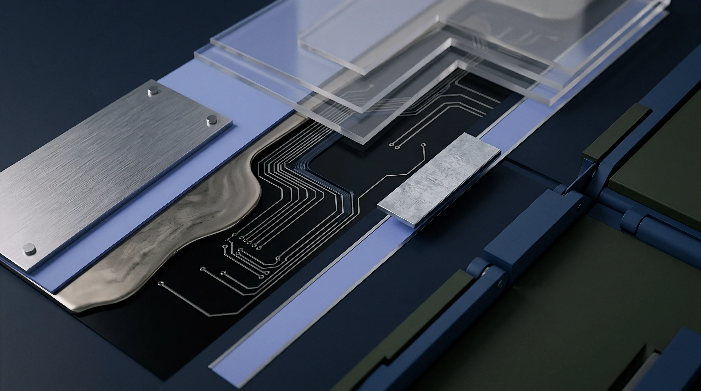
Evaluating vertical z-axis permittivity requires test setups where field lines run perpendicular to the laminate. The Clamped Stripline Resonator method (IPC-TM-650 Method 2.5.5.5) is the standard industry technique for z-axis substrate qualification. Two unclad dielectric cards are clamped between grounded metallic plates around a thin central resonator card with an etched copper pattern.
Hydraulic pressure clamps the assembly to collapse internal air gaps.
Microscopic air gaps between clamped cards and the central resonator pattern are the main source of error in clamped stripline testing. Air carries a relative permittivity of 1.0, so even a one-micrometer air film lowers the measured composite value below the true material property. To suppress air gap errors, IPC-TM-650 Method 2.5.5.5 mandates a standard clamping pressure ~ typically 1.4 megapascals ~ to squeeze out air during measurement.
Other high-frequency approaches use Full Sheet Resonators (FSR) or microstrip ring resonators etched right on production panels. IPC-TM-650 Method 2.5.5.14 covers the FSR technique, treating an entire double-clad sheet as an open-sided cavity. By reading spatial standing wave patterns in the copper-clad panel at microwave frequencies, FSR extracts average z-axis permittivity across the whole sheet footprint.
It gives rapid feedback on raw panel quality without cutting coupons or building complex fixtures.
Choosing the right test method comes down to matching fixture field orientation with circuit field topology. Outer microstrip traces send electric fields through both substrate and surrounding air, depending heavily on x-y permittivity. Embedded inner-layer striplines concentrate field energy vertically between reference planes, relying on z-axis numbers.
Fabricators often publish clamped stripline data on datasheets, which yields lower dielectric values than SPDR tests on the same substrate due to anisotropy.
A two-percent coupon impedance offset often occurs when using clamped stripline datasheet numbers to calculate microstrip dimensions without adjusting for differences in field orientation.

Topology
Conductor layout and fiber weave geometry determine how dielectric variations affect signal timing and impedance control. Woven glass fabric is far from uniform ~ it consists of dense glass bundles separated by resin windows. As trace widths shrink for high-density routing, signal conductors approach the structural pitch of the glass weave.
A 75-micrometer trace running across standard fabric repeatedly crosses between high-permittivity glass bundles and low-permittivity resin pockets, creating localized impedance ripples along its run.
Weave pitch and fill density differ sharply among glass styles. Light fabrics use fine filaments woven closely together; heavy styles use thick bundles spaced farther apart. Glass choice dictates dielectric layer rigidity and pressed thickness, but also sets the spatial frequency of dielectric variations.
Picking the wrong glass style for high-speed differential pairs introduces differential skew, eye degradation, and jitter that routing tweaks during layout cannot fix.

Glass Weave Architecture and Fiber Bundle Geometry
Electronic glass fabrics use four-digit style designations like 106, 1080, 2116, 7628, and 3313. These numbers specify warp and weft thread counts per inch along with yarn linear mass density. Style 106 uses fine yarns woven at 56 by 56 threads per inch to create a thin, uniform sheet with small resin windows.
Style 7628 uses heavy yarns at 44 by 31 threads per inch, leaving large open resin windows hundreds of micrometers across.
Structural differences among glass weaves govern the range of spatial dielectric variation across a panel. The table below compares five standard glass styles, detailing weave density, glass content by weight, pressed thickness, and peak-to-peak dielectric variance when impregnated with high-Tg epoxy.
| Glass Weave Style Designation | Weave Density (Warp x Weft per inch) | Nominal Glass Content (Weight %) | Nominal Pressed Thickness (micrometers) | Spatial Dk Window (10 GHz Peak-to-Peak) |
|---|---|---|---|---|
| Style 106 | 56 x 56 | 33% | 33 | 3.50 to 3.75 |
| Style 1080 | 60 x 60 | 47% | 64 | 3.65 to 3.95 |
| Style 2116 | 60 x 58 | 57% | 102 | 3.80 to 4.15 |
| Style 7628 | 44 x 31 | 65% | 175 | 3.95 to 4.40 |
| Style 3313 (Spread Glass) | 60 x 62 | 54% | 80 | 3.85 to 4.02 |
Spread glass fabrics were developed to smooth out spatial dielectric variations. Mechanical spreading uses high-pressure water jets or rollers to flatten glass yarn bundles during weaving, fanning filaments sideways into the open resin windows. Styles like 1035, 1067, 1078, and 3313 are spread versions of traditional weaves.
Flattening yarns into continuous ribbons eliminates resin windows and flattens spatial permittivity across the panel.
Using spread glass reduces spatial dielectric variation, but pushes up substrate costs. Spread glass cloth requires extra processing steps that add a fifteen to thirty percent premium over standard core stock. Designers must weigh whether data rates justify the cost.
Below 5 Gbps, standard glass paired with zig-zag routing often keeps skew under control. At 28 Gbps, 56 Gbps, or higher, spread glass is usually essential to avoid eye closure.
Standard IPC-4101 specifications permit slash sheet compliance testing on composite glass structures without mandating specific individual glass weave styles within the core construction.

Why Does Glass Style Choice Alter Differential Skew?
Differential signaling uses two parallel traces carrying opposite-polarity signals, with the receiver subtracting one from the other to reject common-mode noise. That cancellation depends on identical propagation delay along both lines. If one trace runs over a glass bundle while its partner sits over a resin window, the glass-side signal sees a higher dielectric constant and travels slower.
The two complementary pulses hit the receiver out of alignment.
This phase offset ~ weave-induced differential skew ~ converts differential signal energy into common-mode noise. When skew becomes a sizable fraction of signal rise time, the eye diagram closes horizontally and cuts into receiver timing margins. On long backplane runs using unspread 1080 or 7628 glass, weave skew can exceed fifty picoseconds over thirty centimeters, completely closing eye margins on 28 Gbps NRZ or 112 Gbps PAM4 links.
Layout designers use routing tricks to curb weave skew without changing materials. Rotating the PCB layout relative to the panel weave ensures long traces never run parallel to warp or weft yarns. Routing lines at a 5 to 10 degree angle to the panel edge forces conductors to average across glass bundles and resin windows over short distances.
Alternatively, CAD tools can apply a subtle periodic zig-zag ~ off-grid routing ~ to individual pairs to achieve the same averaging effect across the weave pitch.
Angled routing curbs skew on straight runs, but wastes panel area and complicates component placement. Rotating an entire layout ten degrees on an eighteen by twenty-four inch panel leaves unusable wedge-shaped scrap along the borders. That array rotation drops the count of usable boards per panel, raising the net cost per board.
Engineers have to balance panel waste against the cost premium of specifying spread glass laminates.
Layer registration errors interact with glass weave patterns to create secondary dielectric shifts in dense backplanes. During eight-layer lamination, pin registration tolerances let core layers shift relative to one another by up to fifty micrometers. When adjacent glass weaves are unaligned, overlapping bundles create complex three-dimensional permittivity variations.
That structural misalignment complicates impedance modeling for internal striplines bound by asymmetric prepreg layers.
The choice between specifying spread-glass laminates and using angled trace routing comes down to which strategy delivers higher overall yield across volume production.
Tolerance
Fabrication drawing specs set strict boundaries on electrical performance. Standard commercial boards call for plus or minus ten percent impedance tolerances on single-ended and differential traces. High-speed servers and aerospace backplanes routinely tighten that target to plus or minus five percent.
Holding five percent in volume production requires controlling copper etch tolerances, dielectric thickness, and substrate permittivity across every panel in a build lot.
Across an eighteen by twenty-four inch panel, local shifts in resin content, pressed thickness, and moisture absorption form a broad spatial distribution curve. If permittivity varies by plus or minus 0.2 units around a baseline of 4.0, that material shift consumes nearly half of a five-percent impedance budget before accounting for copper etch or trace width tolerances. Fabricators use tight process controls and coupon mapping to prevent material variations from causing yield hits during final inspection.

Panel Scale Permittivity Mapping Protocols
Mapping dielectric variance across production panels takes systematic spatial sampling. Fabricators place test coupons along the edges and interior layout of panels to monitor quality. However, perimeter coupons suffer from edge-effect processing artifacts like heavy resin squeeze-out and high plating current density, often showing wider dielectric variation than boards in the center of the panel.
Controlling dielectric variance and protecting panel yield requires running through a design-for-manufacture checklist before releasing the stackup:
- Verify Raw Material Slash Sheets to confirm incoming core and prepreg lots fall within tight IPC-4101 dielectric constant windows.
- Map Copper Thieving Patterns symmetrically across internal signal and power layers to balance resin flow during pressing.
- Specify Spread Glass Fabrics for dielectric layers supporting differential channels running above ten gigabits per second.
- Restrict Prepreg Layer Combinations to at most three thin sheets per opening to limit stacked thickness tolerances and resin displacement.
- Position Impedance Coupons inside internal cutout zones, not just along outer margins, to collect representative electrical test data.
- Require Low-Profile Copper Foils on high-frequency inner layers to reduce surface-roughness permittivity shifts and signal loss.
Permittivity mapping across large panels shows distinct patterns driven by lamination mechanics. Platen centers transfer heat differently than outer edges during initial ramp-up. Resin near the panel edges drops in viscosity earlier, causing heavier resin displacement along the perimeter.
Electrical measurements across hundreds of panels confirm that dielectric constant values follow a radial gradient, with higher effective permittivity near the center where resin retention is highest.
Microstrip impedance equations demonstrate how sensitive trace performance is to substrate permittivity shifts. Under Wheeler’s formula, characteristic impedance varies inversely with the square root of effective dielectric constant. A five-percent rise in local permittivity drops trace impedance by roughly two and a half percent.
Keeping a target 50-ohm line within a plus-or-minus 2.5-ohm window means local dielectric constant cannot shift more than 0.20 units from nominal baseline.
The table below shows how key fabrication variables contribute to overall impedance variation on a 50-ohm microstrip trace built on a 100-micrometer substrate with a nominal dielectric constant of 4.00.
| Physical Process Parameter | Nominal Value | Process Variation Window | Impedance Shift (Ohms) | Percentage of 5% Tolerance Budget |
|---|---|---|---|---|
| Substrate Dielectric Constant (Dk) | 4.00 | + / – 0.20 units | + / – 1.25 ohms | 50% |
| Dielectric Thickness (h) | 100 micrometers | + / – 7.5 micrometers | + / – 2.10 ohms | 84% |
| Trace Top Width (w) | 150 micrometers | + / – 12.5 micrometers | + / – 1.80 ohms | 72% |
| Copper Thickness (t) | 35 micrometers | + / – 5.0 micrometers | + / – 0.35 ohms | 14% |
Combining these tolerances via root-sum-square shows that if parameters drift to their limits simultaneously, total impedance variation exceeds ten percent. Since dielectric thickness and trace etching limits are hard to tighten further, controlling permittivity variation is the best lever for holding tight impedance specs. Fabricators sorting raw core stock into narrow dielectric constant bins achieve significantly better yields on tight-tolerance boards.
Impedance Coupon Drift and Yield Accounting
Verifying finished panels relies on Time-Domain Reflectometry (TDR) testing of coupons on the panel margins. TDR sends a fast voltage step down the coupon trace and reads reflections to calculate impedance along its length. If a coupon fails due to a local dielectric anomaly, the fabricator faces a dilemma: under IPC-6012 rules, a single failed coupon justifies scrapping every board harvested from that panel.
Coupon failures get expensive fast on high-layer-count multilayers. A 16-layer backplane panel measuring eighteen by twenty-four inches can represent thousands of dollars in raw materials, press time, and gold finish. If an edge coupon fails TDR while center production boards meet all physical specs, the fab takes a direct yield hit.
That risk prompts shops to push for coupon-averaging notes on drawings so secondary coupons can be tested before scrapping a whole panel.
Scrap rates reflect material uncertainty: fabricators build risk buffers directly into unit pricing. If a drawing calls for five-percent impedance tolerance without specifying laminate grades, the fab may bump its scrap factor from three percent up to fifteen percent or more. That buffer inflates unit prices.
Specifying tight-tolerance low-loss laminates and granting wider etch windows on non-critical layers cuts fabricator yield risk, bringing down landed board costs.
Production data shows dielectric constant variation follows a normal distribution within a material batch, but splits into a bimodal distribution when different prepreg lot numbers are mixed in a press load. Fabricators that enforce strict lot control ~ using prepreg and core material drawn from single batches ~ eliminate bimodal shifts and stabilize electrical performance.
IPC-6012 Section 3.6.2 mandates that impedance coupons match the exact stackup and trace dimensions of the active board, invalidating TDR results taken from non-conforming coupon geometries.


Contract
Dielectric stability requirements must be explicitly codified in procurement documents to bind the fab shop. Relying on general drawing notes or generic slash sheet references leaves buyers vulnerable to unannounced material changes. Substrate vendors frequently adjust resin chemistry or swap glass weaves to optimize factory throughput, so long as the material meets the broad envelope of the specified IPC-4101 slash sheet.
Those changes can shift high-frequency dispersion and permittivity without violating baseline material specs.
Contractual control starts with precise fabrication notes on the master drawing. The drawing must specify the substrate vendor, product series, glass weave style for every prepreg layer, target dielectric constant, and required test standard. Broad notes like ‘FR-4 High-Tg’ let fabricators quote low-cost commodity laminates with wide spatial dielectric variance and poor lot consistency.
Naming specific material families locks the supplier into proven performance profiles.

Slash Sheet Specifications versus Delivered Panel Yield
IPC-4101 slash sheets group materials by glass transition temperature, decomposition point, and chemical system. IPC-4101/126, for instance, covers high-Tg halogen-free epoxies with a maximum dissipation factor of 0.010 and a nominal dielectric constant window. But the standard permits vendors to report permittivity at any single frequency between 1 MHz and 10 GHz using any approved IPC-TM-650 test method.
That flexibility creates loopholes where two laminates under the same slash sheet show noticeably different dispersion curves.
Buyers close these spec gaps by maintaining an internal master material specification that supplements IPC slash sheets. This document tightens allowable bands for raw core permittivity, mandates specific test procedures (such as SPDR at 10 GHz), and caps lot-to-lot drift. Referencing this master spec in purchase orders stops fab shops from introducing alternative materials without engineering review and written approval.
Disputes over material substitution often hinge on ambiguous verification criteria. If a drawing calls out a dielectric constant of 4.0 plus or minus 0.05 without specifying test frequency or sample conditioning, a supplier can demonstrate compliance by testing dry core stock at 1 MHz. Tested at 10 GHz under ambient humidity, that same core might read 4.25 and fail circuit requirements.
Explicitly stating test conditions in drawing notes eliminates that ambiguity.
Fabrication Drawing Notes for Permittivity Bounds
Stackup notes must clearly govern both physical dimensions and electrical targets. A thorough stackup drawing specifies target dielectric thickness, copper foil type, trace geometry, target impedance, and maximum allowable permittivity drift across the panel. The following notes provide a template for high-speed multilayer documentation:
Note 1: Material Specification All core and prepreg layers shall conform to IPC-4101/126. Baseline substrate material shall be Panasonic Megtron 6 or engineered equivalent approved in writing. Unannounced substitution of resin matrix, ceramic filler content, or glass weave style is strictly prohibited.
Note 2: Glass Weave Architecture Dielectric layers supporting controlled impedance traces on Layers 1, 3, 6, and 8 shall utilize mechanically spread glass fabrics (Styles 1078 or 3313). Standard un-spread glass fabrics (Styles 106, 1080, or 7628) are forbidden on these signal layers.
Note 3: Dielectric Constant Limits Relative dielectric constant (Dk) shall be 3.70 plus or minus 0.05 when measured at 10 GHz in accordance with IPC-TM-650 Method 2.5.5.13 (SPDR). Z-axis relative dielectric constant shall not exceed 3.80 when tested per IPC-TM-650 Method 2.5.5.5 (Clamped Stripline).
Note 4: Controlled Impedance Auditing Finished board trace impedance shall meet target values within plus or minus five percent. Verification shall be performed via TDR coupon testing on every manufactured panel. Test data reports shall be delivered with each production shipment dossier.
Clear drawing notes protect buyers during lot qualification and receiving inspection. If a shipment fails TDR impedance testing, explicit drawing terms provide clear proof of non-compliance rather than relying on vague industry norms. That clarity simplifies warranty claims, enforces supplier accountability, and ensures the fabricator absorbs the cost of scrap panels caused by uncontrolled material variance.
Master supply agreements with audit rights let buyers inspect raw material inventory and lamination press logs on site. Press logs show whether temperature ramp rates and platen pressures stay consistent across production runs, while storage inspections confirm prepreg rolls remain in climate-controlled rooms before kitting. Operational audits confirm the fabricator maintains the process controls needed for stable dielectric performance across volume builds.
Bare board unit pricing reflects the fabricator’s perceived yield risk. Defining stackup details, material specifications, and electrical tolerances with test-report exactness removes vendor pricing hedges, yielding tighter quotes and more reliable long-term supply.